

As we enter an era where intelligent systems are increasingly relied upon to make key decisions, responsible AI has become more critical than ever before. It’s not enough to simply rely on data-driven decision-making; we must also ensure that these systems are fair and just. But how can we do this when the same bias and unfairness that exists in our society is reflected in these very algorithms?
The consequences of biased algorithms are far-reaching and can be devastating. They can perpetuate discriminatory practices, deny individuals opportunities or services, and lead to a range of negative outcomes. It’s no longer just a moral obligation to avoid perpetuating inequalities; it’s a necessity to prevent negative consequences such as reputational damage and legal repercussions.
This article aims to drive home the importance of fairness in AI and provide practical tips for ensuring that algorithms are unbiased and free from discrimination. We will delve into the fairlearn library, a powerful open-source toolkit, to assess and mitigate bias in machine learning. Using fairlearn, we will implement a classification model in Python to predict income on the adult consensus set and evaluate its fairness.
Think about it: just as we strive to ensure fairness in our daily lives, we must also do the same with AI. We must do our best to eliminate bias and discrimination from our algorithms, just as we work to eliminate these issues from our society. By using fairlearn, we can ensure that our models are as fair and unbiased as possible, minimizing the risk of perpetuating discrimination and inequality. We can take steps to ensure that our algorithms are not influenced by factors such as race, gender, or age, and that they are making predictions based on merit alone.
What is Responsible AI?
Responsible AI is an approach that emphasizes fairness, transparency, accountability, and ethical considerations in the development and deployment of AI systems. It involves identifying potential sources of bias in AI and taking steps to address them proactively. To ensure responsible AI, organizations must develop policies and processes that prioritize fairness, transparency, and accountability throughout the AI development lifecycle.
How Real-World Bias Manifests in Biased Data
As we continue to develop increasingly sophisticated AI models like GPT-4, it is crucial to acknowledge that real-world data is not always objective and unbiased. Training models on biased data can lead to the perpetuation and even amplification of existing biases and disparities. Failing to address these issues can cement and exacerbate existing inequalities, with far-reaching consequences for society and individuals alike.
Bias in AI models often stems from the data they are trained on. Historical data, social norms, and cultural practices can all introduce bias into datasets, which AI models may then unwittingly learn and propagate. This can lead to AI systems making biased decisions, producing biased content, or perpetuating stereotypes and prejudices.
Ways in which AI systems can be biased
There are many ways in which AI systems can be biased and thus behave unfairly, including the following:
- Gender Bias in Hiring: The data used by companies to train their hiring algorithms may be biased against certain genders or demographics. As a result, these algorithms may perpetuate existing gender inequalities by disproportionately rejecting female candidates.
- Racial Bias in Healthcare: Medical data may be biased against certain racial or ethnic groups, which can lead to misdiagnosis, mistreatment, or under-treatment of certain populations. For instance, studies have shown that Black patients are less likely to receive appropriate pain management than white patients.
- Economic Bias in Credit Scoring: Financial data used to determine credit scores may be biased against low-income individuals or marginalized communities, making it harder for them to access credit or loans. The result is a cycle of poverty, where individuals cannot access credit and are thus unable to build wealth.
- Age Bias in Predictive Policing: Predictive policing algorithms may be biased against certain age groups, such as younger people, who may be more likely to be falsely flagged as potential criminals. This can lead to increased surveillance and potential harassment of certain populations.
These examples highlight the importance of identifying and addressing bias in real-world data. By doing so, we can ensure that our models and algorithms are fair, just, and equitable for all individuals, regardless of their background or demographic.

Model Fairness and Performance
In machine learning models, there is often a delicate balance between fairness and performance. For instance, optimizing a model for high accuracy might inadvertently lead to discrimination against certain groups of people. To avoid these adverse effects, we must actively work to reduce the influence of unfairness and bias in our models.
Achieving this balance involves multiple strategies, such as gathering diverse and representative data, identifying and addressing sources of bias within the data, and devising techniques to counteract the effects of bias. Moreover, it’s essential to consistently monitor and evaluate our models to ensure they maintain fairness and impartiality over time.
Conversely, when prioritizing fairness, some degree of accuracy may be sacrificed. Striking the right balance between fairness and performance depends on the specific use case and consideration of the potential consequences of any decisions made. The ultimate goal is to create a model that is both fair and effective in performing the task it was designed for.
In summary, to create a well-balanced machine learning model, it’s crucial to acknowledge the trade-off between fairness and performance. By employing various strategies, such as using diverse data, addressing bias, and continuously monitoring the models, we can work towards developing models that are not only accurate but also fair and equitable for all users.

Assessing Model Fairness with the Fairlearn Library
Fairlearn is an open-source Python package, developed by Microsoft, that offers tools for assessing and mitigating unfairness in machine learning models. The library empowers developers and data scientists to pinpoint and address potential sources of bias in their data and models, ensuring that predictions and decisions are made fairly and transparently.
Fairlearn encompasses a variety of algorithms and metrics for evaluating and mitigating unfairness, including:
- Group Fairness: This metric measures the difference in a model’s performance across various subgroups of the population, such as race or gender.
- Demographic Parity: This metric works to ensure that the model’s predictions are distributed fairly across different subgroups of the population.
- Equalized Odds: This metric guarantees that the model’s predictions maintain equal accuracy across different subgroups of the population.
In addition to these metrics, Fairlearn also offers various techniques for mitigating unfairness. These include reweighing data to balance different subgroups, adjusting the model’s predictions to meet specific fairness criteria, and enforcing fairness constraints during the training process. By utilizing Fairlearn, developers and data scientists can be confident that their machine learning models are more equitable and unbiased.

Mitigating Unfairness in Machine Learning
There are two options to address unfairness in machine learning models: consider fairness during training or add a post-processing step to mitigate unfairness as an additional layer. Both methods have their merits and drawbacks. The ideal approach depends on the context and objectives of the problem you’re tackling.
Considering fairness during training involves incorporating fairness constraints into the learning process. This approach can lead to more interpretable models, as fairness is embedded from the start. However, it may require specialized algorithms and could result in reduced performance.
On the other hand, adding a post-processing step to mitigate unfairness involves adjusting the model’s predictions after training. This method offers flexibility, as it can be applied to any pre-trained model. It may also preserve performance better. However, it might not provide as much interpretability, as fairness is addressed separately from the original model.
Ultimately, the choice depends on your specific goals, the model’s purpose, and the importance of interpretability versus performance.
Considering Fairness during Training with Fairness Constraints
Considering fairness during training involves incorporating fairness constraints or objectives into the model’s training process. This can be done in different ways:
- by balancing the training dataset to ensure equal representation of different groups.
- by adjusting the model’s loss function to penalize unfair predictions,
- or by adding fairness constraints to the optimization problem.
The main advantage of this approach is that it can lead to models that are inherently fair without requiring any additional post-processing steps. However, it can be challenging to define and operationalize fairness. In addition, the fairness objectives may conflict with other objectives, such as accuracy or generalization.
There are several fairness constraints that can be used to ensure that machine learning models and decision-making processes do not discriminate against certain groups. Some of the most commonly used constraints include:
- Demographic Parity: This constraint ensures that the proportion of positive outcomes is equal across different demographic groups.
- Equalized Odds: This constraint ensures that the true positive rate and false positive rate are equal across different demographic groups.
- Disparate Impact: This constraint ensures that the ratio of positive outcomes to the total number of outcomes is the same across different demographic groups.
For a full list of constraints, please view the library documentation.
The choice of fairness constraint depends on the specific context and goals of the decision-making process, and the constraints may need to be customized or combined to achieve the desired level of fairness.
Fairness Mitigation as a Postprocessing Layer
Another approach is to add a post-processing step to mitigate the unfairness of existing models. This method involves applying a fairness algorithm to the model’s outputs after training. Examples include reweighting predictions to ensure equal treatment of different groups, calibrating the model’s scores to remove bias, or using a fairness metric to adjust predictions.
The primary advantage of this approach is its applicability to existing models without the need for retraining. However, it might not tackle the root causes of unfairness in the model, and the fairness algorithm could introduce its own biases or trade-offs.
Building A More Inclusive Machine Learning Model using FairLearn and Python
Let’s explore building a fair machine learning model using the census dataset, which includes demographic attributes to predict if a person earns more or less than $50k per year. As income prediction is sensitive, we’ll ensure fairness in our model.
We’ll create an initial fairness-unaware model, evaluate its fairness, and then use grid search to identify alternative models with varying performance and unfairness. This process consists of:
- Load the data: Load the census dataset containing demographic attributes like age, education level, race, and gender.
- Initial preprocessing and visualization: Preprocess the data by removing missing values, encoding categorical variables, scaling numerical features, and visualizing the data for insights.
- Splitting and scaling the data: Split the data into training and testing sets and scale the features to make them comparable.
- Training a fairness-unaware model and assessing fairness: Train a baseline model unaware of unfairness and evaluate its fairness using metrics like disparate impact and statistical parity difference.
- Mitigating bias by training fairness-aware models with fairness constraints: Train models using demographic parity as a fairness constraint to mitigate bias and improve fairness.
- Comparing the performance of the models: Compare the models’ performance in accuracy, fairness, and other metrics like false positives and false negatives.
By following these steps, we’ll build a fair machine learning model that is accurate, equitable, and just.
The code is available on the GitHub repository.

Prerequisites
Before starting the coding part, make sure that you have set up your Python 3 environment and required packages. This will ensure a seamless learning experience and prevent any potential roadblocks or issues that may arise due to an improperly configured environment.
If you don’t have an environment, follow this tutorial to set up the Anaconda environment.
Make sure you install all required packages. In this tutorial, we will be working with the following packages:
- Pandas
- NumPy
- Matplotlib
- Seaborn
- Plotly
- Fairlearn
You can install the Fairlearn library and other packages using console commands:
pip install <package name>
conda install <package name> (if you are using the anaconda packet manager)
About the Adult Consensus Dataset
The Adult Consensus Dataset is a highly regarded and extensively used resource in machine learning and statistics, offering a comprehensive view of over 32,000 individuals across the United States. This invaluable dataset features 14 unique attributes, such as age, education, occupation, work class, marital status, and gender, among others. It also includes a binary target variable, identifying individuals earning over $50,000 annually.
However, the dataset presents challenges, as it contains sensitive demographic features like race and gender. If not handled properly, these features may lead to biased predictions and unfair outcomes. As a result, models trained on this dataset require careful design and evaluation to prevent perpetuating or amplifying existing biases and discrimination.
Despite its complexities, the Adult Consensus Dataset remains a popular choice for training and testing binary classification models. Its value extends further, serving as an excellent benchmark for testing and showcasing fair AI models. The dataset raises important questions about fairness, bias, and discrimination in machine learning, making it an essential resource for creating ethical and unbiased AI solutions.
Step #1 Load Preprocess the Data
We begin by loading the data using the fetch_openml function, making the necessary imports, and performing some initial preprocessing. The dataset is loaded into two data frames, X_df and y_df, where X_df contains the features and y_df contains the binary target variable, which is income with classes “>50k” and “<=50k”. The code below encodes these classes with 0 and 1.
Assessing model fairness is always done with respect to one or several sensitive variables. Although there are several features in the dataset that could be considered sensitive, optimizing the model to consider all of these features simultaneously would lead to significant complexity and increase training times. Therefore, in this tutorial, we will focus specifically on assessing model fairness with respect to sex and race. The sex feature contains two classes, “male” and “female,” while the race feature contains classes for “Black,” “White,” and several further classes.
# A tutorial for this file will be shortly available at www.relataly.com
# Tested with python 3.9.13, matplotlib 3.6.2, numpy 1.23.3, seaborn=0.12.1, fairlearn=0.8.0, plotly 5.11.0

from sklearn.tree import DecisionTreeClassifier
from sklearn.model_selection import train_test_split
from sklearn.preprocessing import LabelEncoder, StandardScaler
from sklearn import metrics as skm
from fairlearn.metrics import MetricFrame, selection_rate, selection_rate_difference, count, plot_model_comparison
from fairlearn.reductions import DemographicParity, ErrorRate, GridSearch
import seaborn as sns
import pandas as pd
import matplotlib.pyplot as plt
sns.set_style('white', { 'axes.spines.right': False, 'axes.spines.top': False})

# read the adult data
# predict whether income exceeds $50K/yr based on census data. Also known as "Census Income" dataset.
# https://archive.ics.uci.edu/ml/datasets/adult

from sklearn.datasets import fetch_openml
data = fetch_openml(data_id=1590, parser='auto', as_frame=True)

X_df = data.data.copy()
data.target = data.target.replace({' <=50K': 0, ' >50K': 1})
y_df = data.target

# Declare sensitive features
sensitive_variables = ["sex", 'race']

# join X_df and y_df and name y_df as 'income'
X_df['salary >50k'] = y_df

# show df that contains the target column
X_df.head()
age workclass fnlwgt education race sex ... hours-per-week salary >50k 0 25 4 226802 1 Black Male ... 40 0 1 38 4 89814 11 White Male ... 50 0 2 28 2 336951 7 White Male ... 40 1 3 44 4 160323 15 Black Male ... 40 1 4 18 0 103497 15 White Female ... 30 0
Step #2 Initial Preprocessing and Visualization
Let’s continue with some initial preprocessing and data visualization. First, we encode the categorical features in the X_df data frame using the LabelEncoder function from scikit-learn. This is important, as the fairlearn gridsearch technique that we will use in this tutorial only works with numeric features.
Next, to simplify the tutorial and reduce model training time, we will filter the dataset to only include people of races “Black” and “White.” This will result in four sensitive feature permutations:
- Black, Woman
- Black, Man
- White, Woman
- White, Man
Finally, we create two data frames. The X_df data frame contains the features we will be using to train our model, but it does not contain the target label anymore. The other data frame, df_visu, does contain the target label and will be used for visualization purposes. Finally, we use df_visu to visualize how the target variable is distributed with respect to our sensitive features.
# encode the categorical features
X_df['workclass'] = X_df['workclass'].cat.codes
X_df['education'] = X_df['education'].cat.codes
X_df['marital-status'] = X_df['marital-status'].cat.codes
X_df['occupation'] = X_df['occupation'].cat.codes
X_df['relationship'] = X_df['relationship'].cat.codes

# filter some values to reduce tutorial complexity and make it easier to visualize
X_df = X_df.loc[X_df["race"].astype(str).isin([" White", " Black"])]
X_df.race = X_df.race.cat.remove_unused_categories()

# ensure that the target column has the same filter applied
y_df = X_df['salary >50k']

# create a copy of the df for visualization
df_visu = X_df.copy()

# drop the target column from X_df
X_df.drop(['salary >50k'], axis=1, inplace=True)

# visualize the distributions of the cateogical variables
fig, ax = plt.subplots(1, 3, figsize=(16, 5))
sns.countplot(x='sex', hue='salary >50k', data=df_visu, ax=ax[0])
sns.countplot(x='race', hue='salary >50k', data=df_visu, ax=ax[1])
sns.kdeplot(x='age', hue='salary >50k', data=df_visu, ax=ax[2])

# rotate x_labels
plt.sca(ax[1])
plt.xticks(rotation=30)
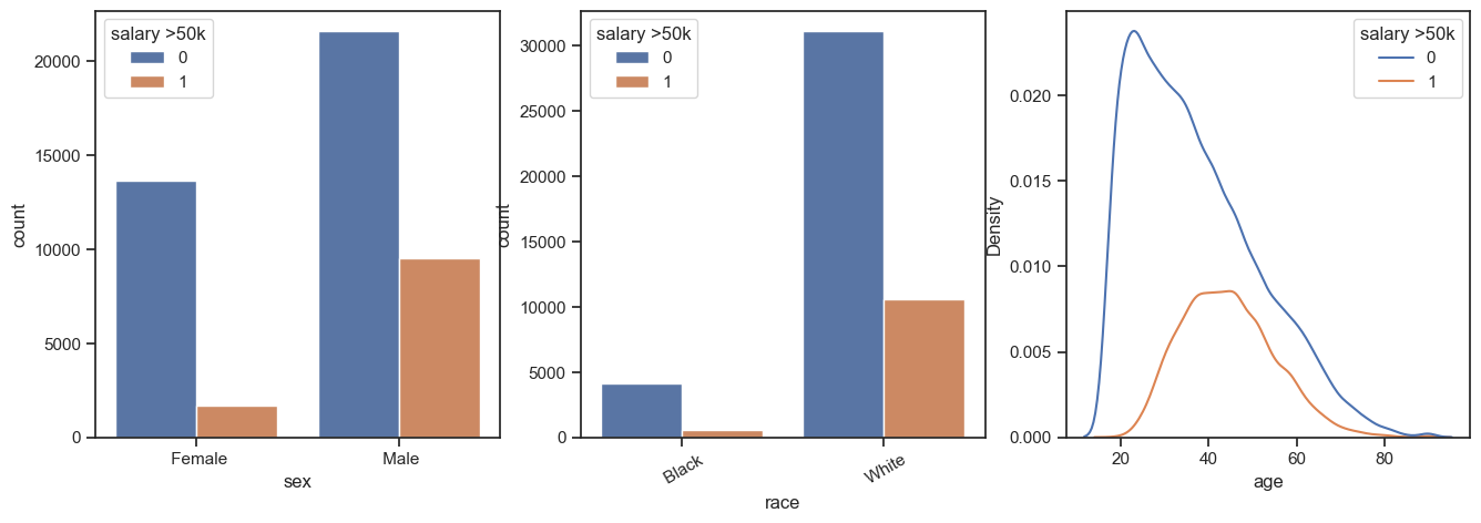
All three plots reflect inequality in our society:
- The percentage of women with a yearly income above 50k is much lower than that of men.
- With respect to race, this bias is even more extreme, with way more white people earning more than 50k than black people.
- Although we won’t use age as a sensitive label, it is noteworthy that the percentage of people earning more than 50k declines with growing age.
Step #3 Splitting and Scaling the Data
The code performs several preprocessing steps. First, the data is split into the features (X_df) and the target variable (y_df). Next, the categorical features in X_df are encoded using the LabelEncoder function from scikit-learn. The data is then split into training and test sets. Records are stratified based on the target variable to ensure that the proportion of each class is maintained in both sets.
It is important to note that the sensitive variables, sex and race, are included in the splitting process to ensure that the data is divided in a fair manner. Specifically, we create a new data frame A containing only the sensitive variables. We then split the data into training and test sets using the stratify parameter based on Y_encoded (the encoded version of y_df) and A.
Finally, the features in X_df are scaled using the StandardScaler function from scikit-learn to ensure that all features are on the same scale. The resulting scaled features are then converted back into a pandas data frame, X_scaled.
# create a dataframe with sensitive features
A = X_df[sensitive_variables]
X = X_df.drop(labels=sensitive_variables, axis=1)
X = pd.get_dummies(X)

# Scale the data
sc = StandardScaler()
X_scaled = sc.fit_transform(X)
X_scaled = pd.DataFrame(X_scaled, columns=X.columns)

# Encode the target variable
le = LabelEncoder()
Y_encoded = le.fit_transform(y_df)

# We split the data into training and test sets:
X_train, X_test, Y_train, Y_test, A_train, A_test = train_test_split(
    X_scaled, Y_encoded, A, test_size=0.4, random_state=0, stratify=Y_encoded
)

# Work around indexing bug
X_train = X_train.reset_index(drop=True)
A_train = A_train.reset_index(drop=True)
X_test = X_test.reset_index(drop=True)
A_test = A_test.reset_index(drop=True)
Step #4 Train a Fairness-Unaware Model and Assess its Fairness
Now it’s time to train our first model. This initial model will be entirely fairness unaware, meaning its predictions will reflect any patterns of unfairness present in the data.
Model training
We’ll begin by training a baseline fairness unaware decision tree classifier with default settings. The model will be trained on the training set (X_train and Y_train) and then tested on the test set (X_test and Y_test).
# Define evaluation metrics for performance and fairness
performance_metric = skm.accuracy_score
fairness_metric = selection_rate_difference

unmitigated_predictor = DecisionTreeClassifier(random_state=0)
unmitigated_predictor.fit(X_train, Y_train)
Evaluation and Visualization
To evaluate the model’s performance, we’ll use two crucial metrics: the accuracy score and the “selection rate difference”. The latter is a vital fairness metric that measures the difference between selection rates of two distinct groups for a specific outcome or prediction.
In machine learning, this metric often helps determine the fairness of a model, especially with sensitive features like race, gender, or age. A selection rate difference of zero indicates that the model is making predictions fairly and without bias, as both groups have equal selection rates.
However, we must pay attention to a positive or negative selection rate difference. It implies that the model is favoring one group over the other, which could signal bias or discrimination. Carefully monitoring this metric is critical to ensure the model is performing fairly and justly.
Lastly, we’ll visualize the results in a bar chart using the accuracy and selection rate by group. This visualization will provide a comprehensive view of the model’s performance and fairness, allowing us to make informed decisions about potential improvements or adjustments needed to strike the right balance between accuracy and fairness.
metric_frame = MetricFrame(
    metrics={
        "accuracy": performance_metric,
        "selection_rate": fairness_metric,
        "count": count,
    },
    sensitive_features=A_test,
    y_true=Y_test,
    y_pred=unmitigated_predictor.predict(X_test),
)

# plot the metrics
print(metric_frame.overall)
print(metric_frame.by_group)
metric_frame.by_group.plot.bar(
    subplots=True,
    layout=[1, 3],
    legend=False,
    figsize=[12, 4],
    title="Accuracy and selection rate by group",
)
accuracy              0.854136
selection_rate        0.197373
count             18579.000000
dtype: float64
                accuracy  selection_rate    count
sex     race
 Female  Black  0.948665        0.053388    974.0
         White  0.921083        0.083873   5246.0
 Male    Black  0.877378        0.161734    946.0
         White  0.813371        0.264786  11413.0
array([[<AxesSubplot: title={'center': 'accuracy'}, xlabel='sex,race'>,
        <AxesSubplot: title={'center': 'selection_rate'}, xlabel='sex,race'>,
        <AxesSubplot: title={'center': 'count'}, xlabel='sex,race'>]],
      dtype=object)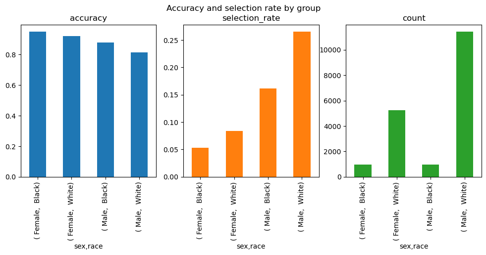
When we look at the selection rate, we can see that the model is intrinsically biased. To be explicit, if this model would go into production, a Black Woman would have a significantly lower chance (5%) to be attributed a +50k income than a White Man (above 25%), even if all other attributes (age, education, and so on) are the same.
Step #5 Train Fairness-Aware Models with Gridsearch
We perform a grid search with demographic parity as a fairness constraint to find the best decision tree classifier model that is both accurate and fair. We evaluate different models with different hyperparameters for the decision tree classifier. The best predictors with the lowest error rates and lowest disparities (in terms of demographic parity) are selected as the dominant models.
We call these models “dominant” because they stand out as superior solutions in multi-objective optimization. “Dominant” implies that these models outshine others across multiple evaluation metrics without falling short in any of the metrics. Dominant models are preferred for their optimal balance of performance and fairness.
During model training, we’ll incorporate demographic parity as a fairness constraint. Demographic parity seeks to ensure equal proportions of positive outcomes (e.g., being hired, approved for a loan, etc.) across various demographic groups (e.g., gender, race, or age) in a population. In simpler terms, it requires the decision-making process not to discriminate against any group based on their demographic characteristics. Mathematically, it’s expressed as P(prediction=1|sensitive_feature=0) = P(prediction=1|sensitive_feature=1), where sensitive_feature is a binary variable indicating membership in a specific demographic group. Achieving demographic parity helps reduce discrimination and promote fairness in decision-making processes. However, depending on the context and goals of the decision-making process, demographic parity might not always be the most appropriate fairness constraint.
Depending on the hardware you are using, training can take several minutes.
# Define and run GridSearch with DemographicParity
sweep = GridSearch(
    DecisionTreeClassifier(random_state=0),
    constraints=DemographicParity(), # DemographicParity() is the default
    grid_size=100, # number of models to evaluate
)
sweep.fit(X_train, Y_train, sensitive_features=A_train)

# The best predictor is the one with the lowest error rate
predictors = sweep.predictors_

errors, disparities = [], []
for p in predictors:

    def classifier(X):
        return p.predict(X)

    # Calculate the error rate of the classifier
    error = ErrorRate()
    error.load_data(X_train, pd.Series(Y_train), sensitive_features=A_train)
    errors.append(error.gamma(classifier)[0])

    # Calculate the disparity in the predictions
    disparity = DemographicParity()
    disparity.load_data(X_train, pd.Series(Y_train), sensitive_features=A_train)
    disparities.append(disparity.gamma(classifier).max())

# Consolidate the results into a single dataframe
grid_results = pd.DataFrame(
    {"predictor": predictors,
     "error": errors,
     "disparity": disparities}
)

# Loop through the grid and select the relevant models
non_dominated_models = []
for model in grid_results.itertuples():
    # only select models with lower disparity compared to the other models
    if model.error < grid_results["error"][grid_results["disparity"] < model.disparity].min():
        non_dominated_models.append(model.predictor)
That’s it; now we have trained several fairness-aware models. Next, let’s look at the performance and fairness of these models.
Step #6 Comparing Dominant and Unmitigated Models
Finally, we’ll evaluate and compare our models’ performance. We’ll assess the dominant models and the unmitigated model using evaluation metrics for performance and fairness. The performance metric we’ll use is the accuracy score, and for fairness, we’ll use the selection rate difference. To do this, we’ll predict on the test data using the unmitigated model, then add predictions for all relevant dominant models.
Next, we’ll create a scatterplot for the models based on their accuracy and selection rate. We’ll use the x-axis for performance metrics and the y-axis for fairness metrics. We’ll also include point labels and display the plot. This visualization will help us understand the trade-offs between performance and fairness in our models.
# We can evaluate the dominant models along with the unmitigated model.

# Use the unmitigated model to predict on the test data
predictions = {"unmitigated_model": unmitigated_predictor.predict(X_test)}

# Add predictions for all relevant dominant models
metric_frames = {"unmitigated_model": metric_frame}
for i in range(len(non_dominated_models)):
    key = "dominant_model_{0}".format(i)
    predictions[key] = non_dominated_models[i].predict(X_test)

    metric_frames[key] = MetricFrame(
        metrics={
            "accuracy": performance_metric,
            "selection_rate": selection_rate,
            "count": count,
        },
        sensitive_features=A_test,
        y_true=Y_test,
        y_pred=predictions[key],
    )

# scatterplot for the models along their accuracy and selection rate
plot_model_comparison(
    x_axis_metric=performance_metric,
    y_axis_metric=fairness_metric,
    y_true=Y_test,
    y_preds=predictions,
    sensitive_features=A_test,
    point_labels=True,
    show_plot=True,
)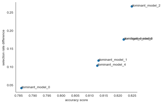
Upon examination, it becomes apparent that we are presented with multiple dominant models that have a marginal difference in their selection rates as well as accuracy levels. These models, while exhibiting slightly lower accuracy, are less influenced by race or gender than the fairness-unaware model. As such, these models may be considered viable candidates for deployment in the model selection process.
It is worth noting, however, that while these models appear to be less prone to bias based on sensitive features, they may still exhibit unfairness towards other features that have not been declared sensitive.
Summary
The significance of responsible AI and fairness in machine learning cannot be overstated. With AI systems becoming increasingly integrated into our lives, it’s essential that we proactively address issues of bias and discrimination.
In this article, we’ve taken a small but vital step towards a more equitable world by developing machine learning models that are fair with respect to sensitive features. Our efforts have been focused on ensuring that our models are less biased and more equitable, using techniques such as reweighting and threshold optimization.
The negative consequences of biased models cannot be ignored. They can lead to discrimination and reputational damage, making it even more important to ensure that our AI systems are fair and just. As AI technology continues to advance, there is an increased need for responsible AI and fairness in AI systems, particularly with the development of more powerful generative models that have the potential to revolutionize various industries.
By taking steps to address issues of bias and discrimination in AI systems, we can ensure that these systems promote positive outcomes and benefit everyone equally. We must strive towards a more equitable and just world through responsible AI and fairness in machine learning.

Sources and Further Reading
- Wikipedia/AI ethics
- Fairlearnwhitepaper
- Fairlearn.org
- ChatGPT helped me revise this article.
- github.com/fairlearn/fairlearn
- Images created with Midjourney AI
Books on Responsible AI and Applied Machine Learning
The links above to Amazon are affiliate links. By buying through these links, you support the Relataly.com blog and help to cover the hosting costs. Using the links does not affect the price.
Great post!