Stock Market Prediction using Multivariate Time Series and Recurrent Neural Networks in Python

Regression models based on recurrent neural networks (RNNs) can learn sequential patterns in time series data. Long short-term memory (LSTM) layers are designed to retain and discard information over a sequence. We can train such models with one feature (univariate forecasting models) or several features (multivariate models). More inputs only help when they add stable information about the target; they do not guarantee better forecasts.

This tutorial uses Python and Keras to build a multivariate LSTM for the NASDAQ Composite. Fifty sessions of Open, High, Low, Close, and Volume changes map to the next Close log return. We reconstruct the next adjusted close and compare it with both last-close persistence and a training-only median-drift forecast.

The remainder of this tutorial proceeds in two parts. We first compare univariate and multivariate time series models. Then we prepare stationary market-change features, split and scale them without future leakage, train with chronological validation, and evaluate 805 held-out sessions. Finally, we create an illustrative horizon-one forecast.

Disclaimer

This article does not constitute financial advice. Stock markets can be very volatile and are generally difficult to predict. Predictive models and other forms of analytics applied in this article only serve the purpose of illustrating machine learning use cases.

Stock market forecasting has become an exciting application for recurrent neural networks.

Univariate vs. Multivariate Time Series Models

Multivariate models and univariate models differ in the number of their input features. While univariate models consider only a single feature, multivariate models use several input variables (features). In stock market forecasting, we can create additional features from price history. Examples are performance indicators such as moving averages, the RSI, or the Sales Volume. We can also include features from other sources, for example, social media sentiment, weather forecasts, etc. Multivariate models that have additional relevant information available have a chance to outperform univariate models. However, this is only true if the features are relevant and are indicative of future price movements.

Preparing data for training univariate models is more straightforward than for multivariate models. If you are new to time series prediction, you might want to look at my earlier articles. These explain how to develop and evaluate univariate time series models:

• Stock Market Forecasting using Univariate Models and Python
• Multi-step Time Series Forecasting with Python: Step-by-Step Guide
• Stock Market Prediction – Adjusting Time Series Prediction Intervals
• Evaluating Time Series Forecasting Models with Python

Univariate Prediction Models

In time series regression, the standard approach is to train a model using past values from the time series that need to be predicted. The assumption is that the value of a time series at time t is closely related to the previous time steps t-1, t-2, t-3, and so on. This approach is similar to chart analysis, which involves identifying patterns in a price chart that can indicate future movements. Both approaches rely on the ability to identify recurring patterns in the data and make accurate predictions based on them. The performance of the model or analysis depends on the ability to identify these patterns and draw the right conclusions from them.

Several techniques can be used to improve the performance of time series regression models, including feature engineering, hyperparameter optimization, and ensemble methods. In addition to these techniques, it is also important to carefully evaluate the performance of the model using appropriate metrics, such as mean squared error or mean absolute error, and to continuously monitor the model’s performance to ensure it remains accurate over time.

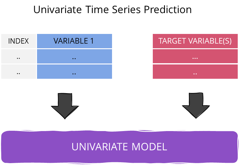
Univariate Time Series Prediction

Multivariate Prediction Models

Predicting the price of a financial asset is a challenging task due to the numerous variables that can influence it, including economic cycles, political events, unforeseen occurrences, psychological factors, market sentiment, and even the weather. These variables are often interdependent, which makes statistical modeling even more complex. While multivariate models can take into account several factors, they are still a simplification of reality and may not fully capture the complexity of the market. On the other hand, univariate models only consider a single dependent variable, ignoring the other dimensions.

Even with good features, predicting financial prices can be difficult because patterns and market rules may change frequently. As a result, models may make mistakes. However, as Georg Box famously said, “All models are wrong, but some are useful.” Despite their limitations, multivariate models can provide a more detailed representation of reality compared to univariate models, and can still be useful in forecasting financial prices.

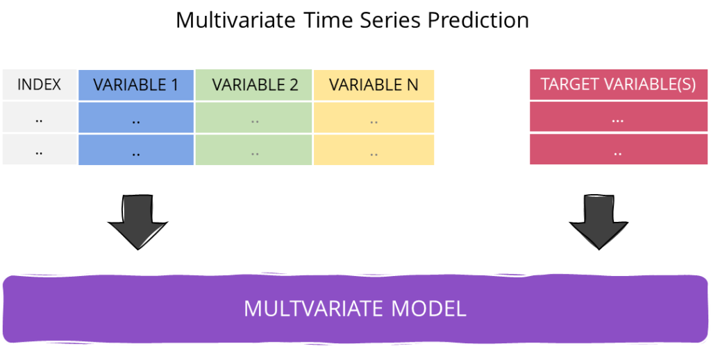
Multivariate Time Series Prediction

Implementing a Multivariate Time Series Prediction Model in Python

Now that we have a solid understanding of multivariate time series forecasting, it’s time to put our knowledge into practice by building a model using Python and TensorFlow. Specifically, we will create a multivariate recurrent neural network (RNN) to predict the NASDAQ stock market index. RNNs are well-suited for time series forecasting because they can process sequential data, considering the dependencies between past and future events.

To build our RNN model, we will need to go through several essential steps.

1. Creating features: We transform price levels and Volume into daily log changes.
2. Splitting and scaling: We split chronologically and fit scalers on training observations only.
3. Sliding window approach: The time series data is sliced into mini-batches using the sliding window approach.
4. Model design and training: The appropriate architecture for the RNN model is chosen, and an optimization algorithm is used to adjust the model’s weights and biases to minimize prediction error.
5. Model validation and predictions: We reserve recent training sequences for validation and keep the test period out of model selection.
6. Reconstruction and evaluation: We invert predicted returns, reconstruct prices, and compare them with simple baselines.

The code is available on the GitHub repository.

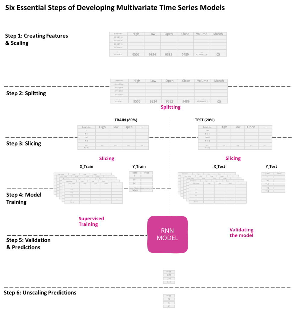
Six Essential Steps for Developing a Multivariate Time Series Model

Prerequisites

Before starting the coding part, make sure that you have set up your Python 3 environment and required packages. If you don’t have a Python environment, follow the steps in this tutorial to set up the Anaconda environment.

Also, make sure you install all required packages. In this tutorial, we will be working with the following standard packages:

• pandas
• NumPy
• matplotlib

In addition, we use Keras with the TensorFlow backend, scikit-learn, seaborn, and yfinance. The refreshed notebook was tested with Python 3.12, TensorFlow 2.21, Keras 3.15, pandas 3.0, scikit-learn 1.9, and yfinance 1.5.

You can install packages using console commands:

• pip install <package name>
• conda install <package name> (if you use the Anaconda package manager)

Step #1 Load the Time Series Data

Let’s start by loading price data on the NASDAQ Composite index (symbol: ^IXIC) from Yahoo Finance with yfinance.

We provide the technical symbol for the index, ^IXIC. A fixed endpoint at the end of 2025 keeps the split, metrics, and illustrative forecast reproducible. auto_adjust=True returns adjusted OHLC prices, and multi_level_index=False preserves a simple single-ticker DataFrame with current yfinance releases.

Running the code below loads the data into a new DataFrame object.

# Time Series Forecasting - Multivariate Time Series Models for Stock Market Prediction
# A tutorial for this file is available at www.relataly.com
# Tested with Python 3.12, TensorFlow 2.21, Keras 3.15, pandas 3.0, and yfinance 1.5

import keras
import matplotlib.dates as mdates
import matplotlib.pyplot as plt
import numpy as np
import pandas as pd
import seaborn as sns
import tensorflow as tf
import yfinance as yf
from sklearn.metrics import mean_absolute_error, root_mean_squared_error
from sklearn.preprocessing import RobustScaler

sns.set_theme(style="white", rc={"axes.spines.right": False, "axes.spines.top": False})
keras.utils.set_random_seed(42)

print(f"TensorFlow version: {tf.__version__}")
print(f"Available GPUs: {len(tf.config.list_physical_devices('GPU'))}")

start_date = "2010-01-01"
end_date = "2026-01-01"
stock_name = "NASDAQ Composite"
symbol = "^IXIC"

df = yf.download(
  symbol,
  start=start_date,
  end=end_date,
  auto_adjust=True,
  multi_level_index=False,
  progress=False,
)
if df.empty:
  raise RuntimeError("yfinance returned no data for the NASDAQ Composite")

print(df.shape)
df.head()

TensorFlow version: 2.21.0
Available GPUs: 0
(4024, 5)

The data looks as expected and has the following columns:

• High - the daily high
• Low - the daily low
• Open - the opening price
• Volume - the daily trading volume
• Close - the adjusted closing level because auto_adjust=True

Step #2 Explore the Data

Let’s first familiarize ourselves with the data before processing them further. Line plots are an excellent choice to gain a quick overview of time series data. By running the code below, we loop over the columns to plot a line chart for each column of the dataframe.

df_plot = df.copy()
_, axes = plt.subplots(nrows=3, ncols=2, sharex=True, figsize=(14, 9))

for ax, column in zip(axes.flat, df_plot.columns):
  sns.lineplot(x=df_plot.index, y=df_plot[column], ax=ax)
  ax.xaxis.set_major_locator(mdates.AutoDateLocator())
  ax.set_title(column)

for ax in axes.flat[len(df_plot.columns):]:
  ax.set_visible(False)

plt.tight_layout()
plt.show()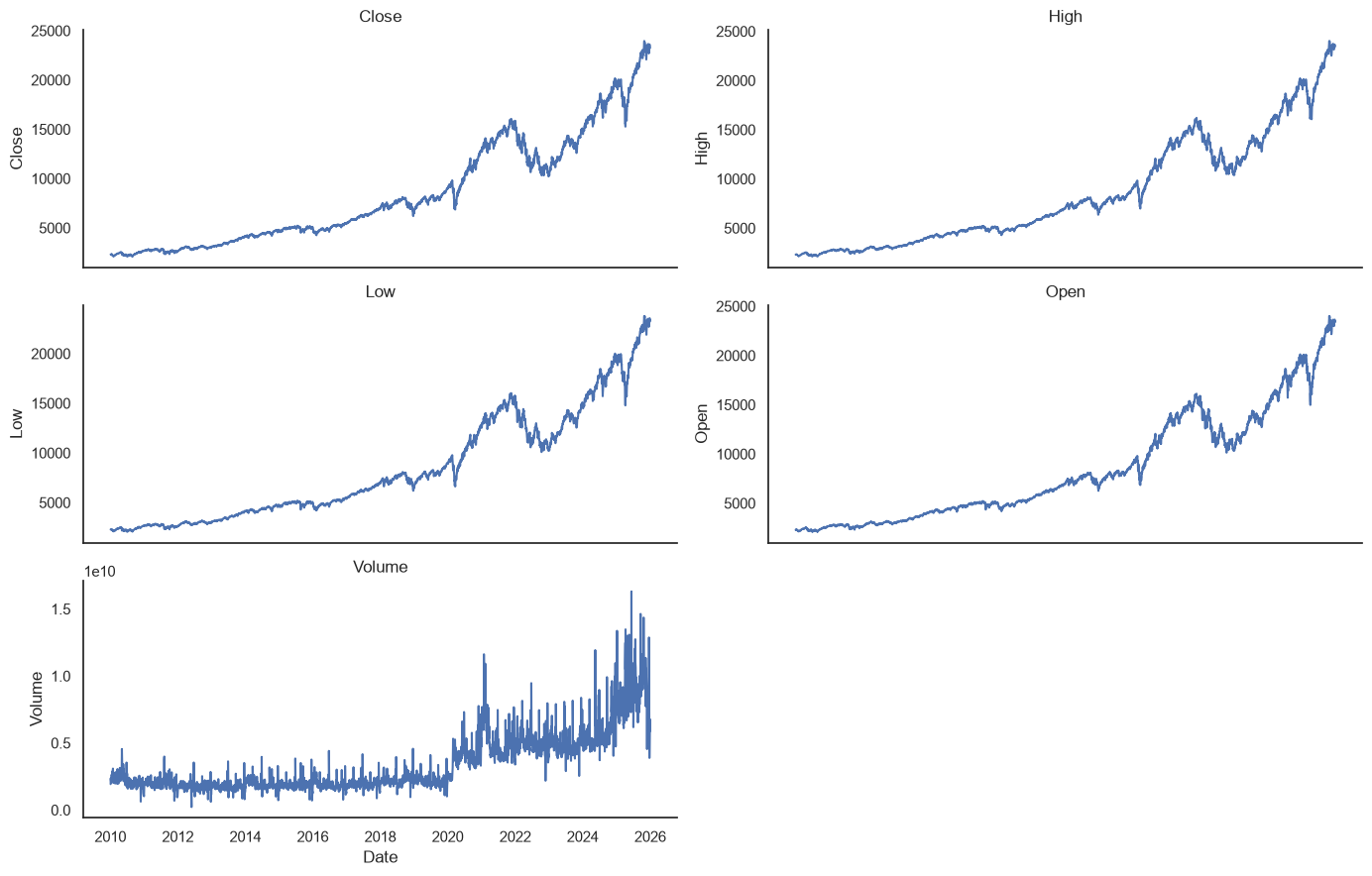

The level plots make the long-term scale change clear: the index rises from roughly 2,300 to above 23,000. This is one reason we model daily changes instead of asking the network to extrapolate raw levels.

Step #3 Feature Selection and Scaling

Before we can train the neural network, we need to transform the data into a processable shape. In this section, we:

• convert OHLC levels and Volume into daily log changes
• split the observations chronologically
• fit separate input and target scalers on the training period only

3.1 Selecting Features

First, we select and transform the features on which we want to train the neural network. Feature engineering is a complex topic, and we could add variables such as moving averages. To keep this example focused, we use the five series already present in our data. To learn more, see the feature engineering tutorial.

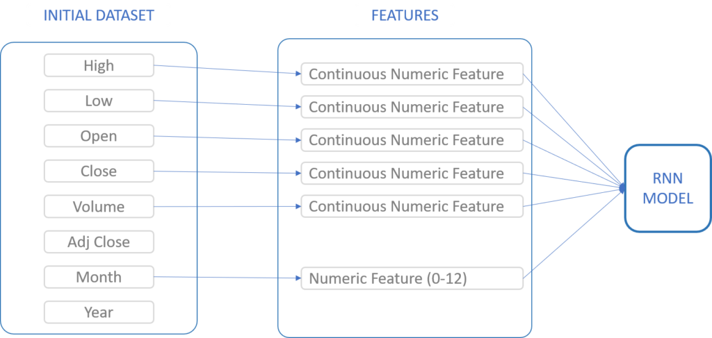
Feature Selection of Multivariate Time Series Models

Raw index levels are non-stationary and change scale substantially over the sample. We calculate one-session log returns for Open, High, Low, and Close, plus the log change in Volume. The target is the next Close log return. We retain the matching Close levels only to reconstruct dollar forecasts later.

market = df.sort_index().dropna().copy()

price_columns = ["Open", "High", "Low", "Close"]
price_log_returns = np.log(market[price_columns]).diff()
volume_log_change = np.log1p(market["Volume"]).diff().rename("Volume")
features = pd.concat([price_log_returns, volume_log_change], axis=1).dropna()

feature_values = features.to_numpy()
close_returns = features[["Close"]].to_numpy()
close_levels = market.loc[features.index, "Close"].to_numpy()
train_size = int(len(features) * 0.8)

print(f"Features: {features.columns.tolist()}")
print(f"Transformed shape: {features.shape}")
print(f"Training rows: {train_size}")
features.tail()

Features: ['Open', 'High', 'Low', 'Close', 'Volume']
Transformed shape: (4023, 5)
Training rows: 3218

3.2 Scaling the Multivariate Input Data

Scaling helps the optimizer handle features with different distributions. We use one RobustScaler for the five inputs and another for the one-dimensional target. Both scalers are fit only on the first 80% of transformed rows. They can then transform later observations without allowing the center or spread of the test period to influence training.

feature_scaler = RobustScaler()
feature_scaler.fit(feature_values[:train_size])
scaled_features = feature_scaler.transform(feature_values)

target_scaler = RobustScaler()
target_scaler.fit(close_returns[:train_size])
scaled_close_returns = target_scaler.transform(close_returns)

print(f"Scaled feature shape: {scaled_features.shape}")
print(f"Feature scaler center: {np.round(feature_scaler.center_, 6)}")
print(f"Target scaler center: {target_scaler.center_[0]:.6f}")

Scaled feature shape: (4023, 5)
Feature scaler center: [ 0.001444  0.001106  0.001260  0.001003 -0.001445]
Target scaler center: 0.001003

Step #4 Transforming the Multivariate Data

Next, we prepare a three-dimensional input structure. Its dimensions represent samples, time steps, and features. We must preserve this shape when using the trained model for a new forecast.

An essential step in the preparation process is slicing the data into multiple input data sequences with associated target values. We write a simple Python script that uses a “sliding window.” This approach moves a window through the time series data, adding a sequence of multiple data points to the input data with each step. The target value (e.g., Closing Price) follows this sequence, and we store it in a separate target dataset. Then we push the window one step further and repeat these activities. This process results in a data set with many input sequences (mini-batches), each with a corresponding target value in the target record. This process applies both to the training and the test data.

Sliding Window

We apply the sliding-window approach to the transformed data. Each input contains 50 sessions and five features; its target is the Close return for the immediately following session. Target positions make the chronological masks explicit. The final training target is before the split, while the first test target is exactly at the split and uses only earlier observations as input.

sequence_length = 50


def create_sequences(feature_values, target_values, sequence_length):
  inputs, targets, target_indices = [], [], []
  for target_index in range(sequence_length, len(feature_values)):
    inputs.append(feature_values[target_index - sequence_length:target_index])
    targets.append(target_values[target_index, 0])
    target_indices.append(target_index)

  return (
    np.asarray(inputs, dtype=np.float32),
    np.asarray(targets, dtype=np.float32),
    np.asarray(target_indices),
  )


x_all, y_all, target_indices = create_sequences(
  scaled_features,
  scaled_close_returns,
  sequence_length,
)
train_mask = target_indices < train_size
test_mask = target_indices >= train_size

x_train, y_train = x_all[train_mask], y_all[train_mask]
x_test, y_test = x_all[test_mask], y_all[test_mask]
test_target_indices = target_indices[test_mask]

print(f"Training shapes: {x_train.shape}, {y_train.shape}")
print(f"Test shapes: {x_test.shape}, {y_test.shape}")

assert target_indices[train_mask][-1] == train_size - 1
assert test_target_indices[0] == train_size
print(
  "First test target:",
  features.index[test_target_indices[0]].date(),
  "using data through",
  features.index[test_target_indices[0] - 1].date(),
)

Training shapes: (3168, 50, 5), (3168,)
Test shapes: (805, 50, 5), (805,)
First test target: 2022-10-17 using data through 2022-10-14

Step #5 Train the Multivariate Prediction Model

Once the data is ready, we can train the model. Its architecture consists of:

• an explicit Keras 3 input for 50 time steps and five features
• an LSTM layer with 32 units
• a dense layer with 16 ReLU units
• one linear output for the scaled next-session Close return

The number of LSTM units is a model choice; it does not need to equal the number of values in an input sequence. This compact network has 5,409 trainable parameters. We optimize Huber loss, which reduces the influence of unusually large return observations relative to mean squared error.

model = keras.Sequential(
  [
    keras.layers.Input(shape=(sequence_length, x_train.shape[2])),
    keras.layers.LSTM(32),
    keras.layers.Dense(16, activation="relu"),
    keras.layers.Dense(1),
  ],
  name="nasdaq_multivariate_lstm",
)
model.compile(
  optimizer=keras.optimizers.Adam(),
  loss=keras.losses.Huber(),
)
model.summary()

The final 10% of training sequences provides chronological validation. The test period remains untouched until final evaluation. We disable shuffling and restore weights from the epoch with the lowest validation loss.

early_stopping = keras.callbacks.EarlyStopping(
  monitor="val_loss",
  patience=3,
  restore_best_weights=True,
)
history = model.fit(
  x_train,
  y_train,
  batch_size=32,
  epochs=20,
  validation_split=0.1,
  shuffle=False,
  callbacks=[early_stopping],
  verbose=1,
)

Let’s take a quick look at the loss curve.

loss_history = pd.DataFrame(
  {
    "Training loss": history.history["loss"],
    "Validation loss": history.history["val_loss"],
  }
)

_, ax = plt.subplots(figsize=(10, 5))
sns.lineplot(data=loss_history, ax=ax)
ax.set_title("Model Loss")
ax.set_xlabel("Epoch")
ax.set_ylabel("Huber loss")
plt.show()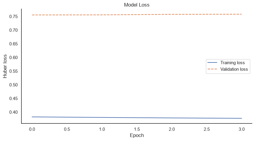

Training stopped after four epochs because validation loss did not improve. The divergence between training and validation loss is an early warning that the historical relationships do not generalize strongly to later training observations. Held-out baselines will provide the more important test.

Step #6 Evaluate Model Performance

Once we have trained the model, we finally use the 805 held-out sessions. We invert the target scaling to recover predicted and actual log returns, then reconstruct each next-session close from the previous close.

Two baselines provide context. Persistence predicts no change. Training-median drift applies the median Close return estimated from training observations only. We compare MAE and RMSE in index points, then check directional accuracy against an always-up rule. For more information on regression metrics, see this article.

predicted_returns_scaled = model.predict(x_test, verbose=0)
predicted_returns = target_scaler.inverse_transform(predicted_returns_scaled).ravel()
actual_returns = target_scaler.inverse_transform(y_test.reshape(-1, 1)).ravel()

origin_prices = close_levels[test_target_indices - 1]
actual_prices = close_levels[test_target_indices]
predicted_prices = origin_prices * np.exp(predicted_returns)
persistence_prices = origin_prices
training_median_return = float(np.median(close_returns[:train_size]))
drift_prices = origin_prices * np.exp(training_median_return)

model_mae = mean_absolute_error(actual_prices, predicted_prices)
model_rmse = root_mean_squared_error(actual_prices, predicted_prices)
baseline_mae = mean_absolute_error(actual_prices, persistence_prices)
baseline_rmse = root_mean_squared_error(actual_prices, persistence_prices)
drift_mae = mean_absolute_error(actual_prices, drift_prices)
drift_rmse = root_mean_squared_error(actual_prices, drift_prices)
directional_accuracy = np.mean(
  np.sign(predicted_returns) == np.sign(actual_returns)
)
up_day_rate = np.mean(actual_returns > 0)

print(f"LSTM MAE: ${model_mae:,.2f}")
print(f"LSTM RMSE: ${model_rmse:,.2f}")
print(f"Persistence MAE: ${baseline_mae:,.2f}")
print(f"Persistence RMSE: ${baseline_rmse:,.2f}")
print(f"Training-median drift MAE: ${drift_mae:,.2f}")
print(f"Training-median drift RMSE: ${drift_rmse:,.2f}")
print(f"LSTM directional accuracy: {directional_accuracy:.1%}")
print(f"Always-up directional accuracy: {up_day_rate:.1%}")

LSTM MAE: $148.99
LSTM RMSE: $212.89
Persistence MAE: $151.35
Persistence RMSE: $213.73
Training-median drift MAE: $149.77
Training-median drift RMSE: $213.25
LSTM directional accuracy: 56.6%
Always-up directional accuracy: 56.8%

The LSTM improves on persistence by 2.36 MAE points and 0.84 RMSE points. Against the more competitive training-median drift baseline, the advantages shrink to 0.78 MAE points and 0.36 RMSE points. These are marginal differences, not evidence of a practically meaningful forecasting edge.

The direction result reinforces that conclusion. The LSTM is correct on 56.6% of sessions, while predicting an increase every session is correct 56.8% of the time. The model therefore does not add directional information beyond the positive-day frequency in this held-out period.

Next, we plot the model and both baselines over the final held-out year. Because each method starts from the previous actual close, all three can look close to the target on a level chart. The aggregate errors and directional comparison above remain the better evidence.

forecast_frame = pd.DataFrame(
  {
    "Actual": actual_prices,
    "LSTM forecast": predicted_prices,
    "Persistence": persistence_prices,
    "Training-median drift": drift_prices,
  },
  index=features.index[test_target_indices],
)
display_start_date = "2025-01-01"
forecast_zoom = forecast_frame.loc[display_start_date:]

_, ax = plt.subplots(figsize=(16, 6))
sns.lineplot(data=forecast_zoom, ax=ax)
ax.set_title("One-Session NASDAQ Forecasts")
ax.set_ylabel("Adjusted close")
ax.set_xlabel("Date")
plt.show()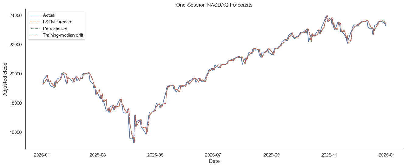

Step #7 Predict the Next Day’s Price

After evaluation, we can generate an illustrative next-session forecast. We pass the latest 50 transformed observations to the model, invert its scaled return, and reconstruct a price from the last adjusted close. We report it beside persistence and training-median drift because the held-out evaluation showed only marginal differences between them.

latest_input = scaled_features[-sequence_length:].reshape(
  1,
  sequence_length,
  scaled_features.shape[1],
)
predicted_return_scaled = model.predict(latest_input, verbose=0)
predicted_return = float(
  target_scaler.inverse_transform(predicted_return_scaled)[0, 0]
)

last_close = float(close_levels[-1])
predicted_close = last_close * np.exp(predicted_return)
drift_close = last_close * np.exp(training_median_return)
forecast_comparison = pd.Series(
  {
    "Last close / persistence": last_close,
    "Training-median drift": drift_close,
    "Illustrative LSTM forecast": predicted_close,
  }
)

print(f"Last observed adjusted close on {features.index[-1].date()}: ${last_close:,.2f}")
print(f"Predicted next-session return: {predicted_return:.3%}")
print(forecast_comparison.round(2).to_string())

Last observed adjusted close on 2025-12-31: $23,241.99
Predicted next-session return: 0.213%
Last close / persistence      23241.99
Training-median drift         23265.32
Illustrative LSTM forecast    23291.46

This output is a demonstration of the inference pipeline, not a recommendation. It can also vary with training randomness unless the full environment is deterministic.

Summary

This tutorial demonstrated multivariate time series modeling for stock market prediction in Python. We trained a compact LSTM that maps 50 sessions of five NASDAQ market-change features to the next Close return. We fitted preprocessing on training data only, used chronological training validation, kept the test period out of model selection, and reconstructed prices for evaluation.

The model achieved an MAE of $148.99, compared with$151.35 for persistence and $149.77 for training-median drift. Its directional accuracy of 56.6% was slightly lower than the 56.8% always-up rate. The model therefore showed no meaningful directional advantage and only a marginal level-error improvement over a simple drift assumption.

Multivariate time series forecasting is a complex topic, and data transformation is often the most important part. Further experiments could add features with information unavailable in OHLCV history, repeat training across random seeds, use walk-forward evaluation, and test whether any improvement survives costs and changing market regimes.

Another interesting approach to stock market prediction uses candlestick images and convolutional neural networks. If this topic interests you, check out the following article: Deep reinforcement learning stock market trading, utilizing a CNN with candlestick images

I am always trying to learn and improve. If you want to give feedback or have remarks, feel free to share them in the comments.

Stockmarket forecasting with a neural network is about identifying meaningful patterns. Be aware that there is no guarantee that these patterns are present in the data. Image created with Midjourney.

Sources and Further Reading

1. Charu C. Aggarwal (2018) Neural Networks and Deep Learning
2. Jansen (2020) Machine Learning for Algorithmic Trading: Predictive models to extract signals from market and alternative data for systematic trading strategies with Python
3. Aurélien Géron (2019) Hands-On Machine Learning with Scikit-Learn, Keras, and TensorFlow: Concepts, Tools, and Techniques to Build Intelligent Systems
4. David Forsyth (2019) Applied Machine Learning Springer
5. Andriy Burkov (2020) Machine Learning Engineering

The links above to Amazon are affiliate links. By buying through these links, you support the Relataly.com blog and help to cover the hosting costs. Using the links does not affect the price.