

Are you interested in learning how multivariate forecasting models can enhance the accuracy of stock market predictions? Look no further! While traditional time series data provides valuable insights into historical trends, multivariate forecasting models utilize additional features to identify patterns and predict future price movements. This process, known as “feature engineering,” is a crucial step in creating accurate stock market forecasts.
In this article, we dive into the world of feature engineering and demonstrate how it can improve stock market predictions. We explore popular financial analysis metrics, including Bollinger bands, RSI, and Moving Averages, and show how they can be used to create powerful forecasting models.
But we don’t just stop at theory. We provide a hands-on tutorial using Python to prepare and analyze time-series data for stock market forecasting. We leverage the power of recurrent neural networks with LSTM layers, based on the Keras library, to train and test different model variations with various feature combinations.
By the end of this article, you’ll have a thorough understanding of feature engineering and how it can improve the accuracy of stock market predictions. So, buckle up and get ready to discover how multivariate forecasting models can take your stock market analysis to the next level!
New to time series modeling?
Consider starting with the following tutorial on univariate time series models: Stock-market forecasting using Keras Recurrent Neural Networks and Python.
Disclaimer: This article does not constitute financial advice. Stock markets can be very volatile and are generally difficult to predict. Predictive models and other forms of analytics applied in this article only illustrate machine learning use cases.

Feature Engineering for Stock Market Forecasting – Borrowing Features from Chart Analysis
The idea behind multivariate time series models is to feed the model with additional features that improve prediction quality. An example of such an additional feature is a “moving average.” Adding more features does not automatically improve predictive performance but increases the time needed to train the models. The challenge is to find the right combination of features and to create an input form that allows the model to recognize meaningful patterns. There is no way around conducting experiments and trying out feature combinations. This process of trial and error can be time-consuming. It is, therefore, helping to build upon established indicators.
In stock market forecasting, we can use indicators from chart analysis. This domain forecasts future prices by studying historical prices and trading volume. The underlying idea is that specific patterns or chart formations in the data can signal the timing of beneficial buying or selling decisions. We can borrow indicators from this discipline and use them as input features.
When we develop predictive machine learning models, the difference from chart analysis is that we do not aim to analyze the chart ourselves manually, but try to create a machine learning model, for example, a recurrent neural network, that does the job for us.
Stock Market Forecasting – Does this really Work?
It is essential to point out that the effectiveness of chart analysis and algorithmic trading is controversial. There is at least as much controversy about whether it is possible to predict the price of stock markets with neural networks. Various studies and researchers have examined the effectiveness of chart analysis with different results. One of the most significant points of criticism is that it cannot take external events into account. Nevertheless, many financial analysts consider financial indicators when making investment decisions, so a lot of money is moved simply because many people believe in statistical indicators.
So without knowing how well this will work, it is worth an attempt to feed a neural network with different financial indicators. But first and foremost, I see this as an excellent way to show how feature engineering works. Just make sure not to rely on the predictions of these models blindly.
Also: Stock Market Prediction using Univariate Recurrent Neural Networks
Selected Statistical Indicators
The following indicators are commonly used in chart analysis and may be helpful when creating forecasting models:
- Relative Strength Index
- Simple Moving Averages
- Exponential Moving Averages
- Bolliger Bands
Relative Strength Index (RSI)
The Relative Strength Index (RSI) is one of the most commonly used oscillating indicators. In 1978, Welles Wilder developed it to determine the momentum of price movements and compare the strength of price losses in a period with price gains. It can take percentage values between 0 and 100.
Reference lines determine how long an existing trend will last before expecting a trend reversal. In other words, when the price is heavily oversold or overbought, one should expect a trend reversal.
- The reference line is at 40% (oversold) and 80% (overbought) with an upward trend.
- The reference line is at 20% (oversold) and 60% (overbought) with a downtrend.
The formula for the RSI is as follows:
- Calculate the sum of all positive and negative price changes in a period (e.g., 30 days):
- We then calculate the mean value of the sums with the following formula:
- Finally, we calculate the RSI with the following formula:


Simple Moving Averages (SMA)
Simple Moving Averages (SMA) is another technical indicator that financial analysts use to determine if a price trend will continue or reverse. The SMA is the average sum of all values within a certain period. Financial analysts pay close attention to the 200-day SMA (SMA-200). When the price crosses the SMA, this may signal a trend reversal. Furthermore, we often use SMAs for 50 (SMA-50) and 100 days (SMA-100) periods. In this regard, two popular trading patterns include the death cross and a golden cross.
- A death cross occurs when the trend line of the SMA-50/100 crosses below the 200-day SMA. This suggests that a falling trend will likely accelerate downwards.
- A golden cross occurs when the trend line of the SMA-50/100 crosses over the 200-day SMA, suggesting a rising trend will likely accelerate upwards.
We can use the SMA in the input shape of our model simply by measuring the distance between two trendlines.
Exponential Moving Averages (EMA)
The exponential moving average (EMA) is another lagging trend indicator. Like the SMA, the EMA measures the strength of a price trend. The difference between SMA and EMA is that the SMA assigns equal values to all price points, while the EMA uses a multiplier that weights recent prices higher.
The formula for the EMA is as follows: Calculating the EMA for a given data point requires past price values. For example, to calculate the SMA for today, based on 30 past values, we calculate the average price values for the past 30 days. We then multiply the result by a weighting factor that weighs the EMA. The formula for this multiplier is as follows: Smoothing factor / (1+ days)
It is common to use different smoothing factors. For a 30-day moving average, the multiplier would be [2/(30+1)]= 0.064.
As soon as we have calculated the EMA for the first data point, we can use the following formula to calculate the ema for all subsequent data points: EMA = Closing price x multiplier + EMA (previous day) x (1-multiplier)
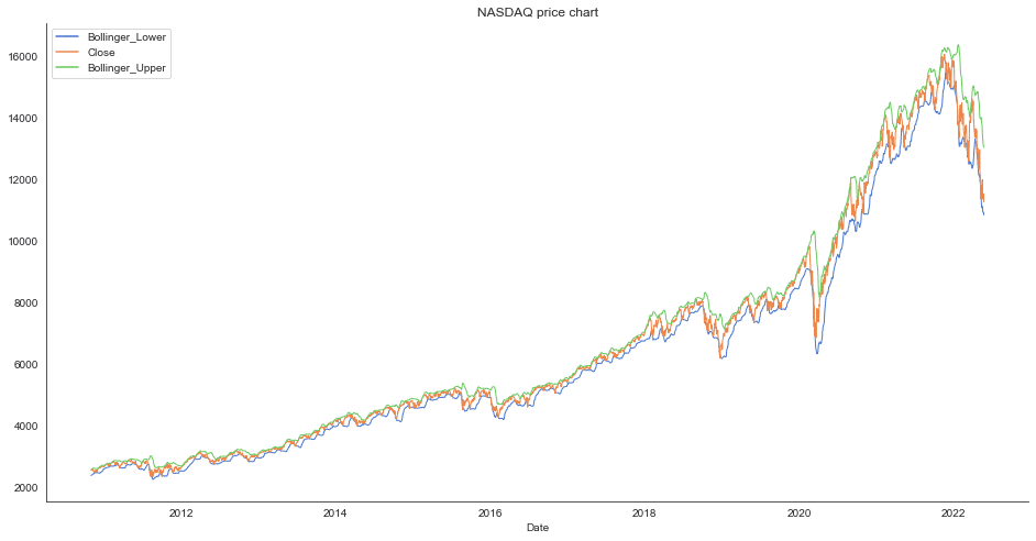
Bollinger Bands
Bollinger Bands are a popular technical analysis tool used to identify market volatility and potential price movements in financial markets. They are named after their creator, John Bollinger.
Bollinger Bands consist of three lines that are plotted on a price chart. The middle line is a simple moving average (SMA) of the asset price over a specified period (typically 20 days). The upper and lower lines are calculated by adding and subtracting a multiple (usually two) of the standard deviation of the asset price from the middle line.
The upper band is calculated as: Middle band + (2 x Standard deviation) The lower band is calculated as: Middle band – (2 x Standard deviation)
The standard deviation is a measure of how much the asset price deviates from the average. When the asset price is more volatile, the bands widen, and when the price is less volatile, the bands narrow.
Traders use Bollinger Bands to identify potential buy or sell signals. When the price touches or crosses the upper band, it may be a sell signal, indicating that the asset is overbought. Conversely, when the price touches or crosses the lower band, it may be a buy signal, indicating that the asset is oversold.
Feature Engineering for Time Series Prediction Models in Python
In the following, this tutorial will guide you through the process of implementing a multivariate time series prediction model for the NASDAQ stock market index. Our aim is to equip you with the knowledge and practical skills required to create a powerful predictive model that can effectively forecast stock prices.
Throughout this tutorial, we will take you through a step-by-step approach to building a multivariate time series prediction model. You will learn how to implement and utilize different features to train and measure the performance of your model. Our goal is to ensure that you are not only able to understand the underlying concepts of multivariate time series prediction, but that you are also capable of applying these concepts in a practical setting.
The code is available on the GitHub repository.

Prerequisites
Before starting the coding part, make sure that you have set up your Python 3 environment and required packages. If you don’t have an environment, follow this tutorial to set up the Anaconda environment.
Also, make sure you install all required packages. In this tutorial, we will be working with the following standard packages:
In addition, we will be using Keras (2.0 or higher) with Tensorflow backend to train the neural network, the machine learning library scikit-learn, and the pandas-DataReader. You can install these packages using the following console commands:
- pip install <package name>
- conda install <package name> (if you are using the anaconda packet manager)
Step #1 Load the Data
Let’s start by setting up the imports and loading the data. Our Python project will use price data from the NASDAQ composite index (symbol: ^IXIC) from yahoo.finance.com.
# Time Series Forecasting - Feature Engineering For Multivariate Models (Stock Market Prediction Example)
# A tutorial for this file is available at www.relataly.com

import math # Mathematical functions
import numpy as np # Fundamental package for scientific computing with Python
import pandas as pd # Additional functions for analysing and manipulating data
from datetime import date # Date Functions
import matplotlib.pyplot as plt # Important package for visualization - we use this to plot the market data
import matplotlib.dates as mdates # Formatting dates
from sklearn.metrics import mean_absolute_error, mean_squared_error # Packages for measuring model performance / errors
import tensorflow as tf
from tensorflow.keras.models import Sequential # Deep learning library, used for neural networks
from tensorflow.keras.layers import LSTM, Dense, Dropout # Deep learning classes for recurrent and regular densely-connected layers
from tensorflow.keras.callbacks import EarlyStopping # EarlyStopping during model training
from sklearn.preprocessing import RobustScaler # This Scaler removes the median and scales the data according to the quantile range to normalize the price data
#from keras.optimizers import Adam # For detailed configuration of the optimizer
import seaborn as sns # Visualization
sns.set_style('white', { 'axes.spines.right': False, 'axes.spines.top': False})


# check the tensorflow version and the number of available GPUs
print('Tensorflow Version: ' + tf.__version__)
physical_devices = tf.config.list_physical_devices('GPU')
print("Num GPUs:", len(physical_devices))

# Setting the timeframe for the data extraction
end_date =  date.today().strftime("%Y-%m-%d")
start_date = '2010-01-01'

# Getting NASDAQ quotes
stockname = 'NASDAQ'
symbol = '^IXIC'

# You can either use webreader or yfinance to load the data from yahoo finance
# import pandas_datareader as webreader
# df = webreader.DataReader(symbol, start=start_date, end=end_date, data_source="yahoo")

import yfinance as yf #Alternative package if webreader does not work: pip install yfinance
df = yf.download(symbol, start=start_date, end=end_date)

# Quick overview of dataset
df.head()
Tensorflow Version: 2.5.0 Num GPUs: 1 [*********************100%***********************] 1 of 1 completed Open High Low Close Adj Close Volume Date 2009-12-31 2292.919922 2293.590088 2269.110107 2269.149902 2269.149902 1237820000 2010-01-04 2294.409912 2311.149902 2294.409912 2308.419922 2308.419922 1931380000 2010-01-05 2307.270020 2313.729980 2295.620117 2308.709961 2308.709961 2367860000 2010-01-06 2307.709961 2314.070068 2295.679932 2301.090088 2301.090088 2253340000 2010-01-07 2298.090088 2301.300049 2285.219971 2300.050049 2300.050049 2270050000
Step #2 Explore the Data
Let’s take a quick look at the data by creating line charts for the columns of our data set.
# Plot line charts
df_plot = df.copy()

ncols = 2
nrows = int(round(df_plot.shape[1] / ncols, 0))

fig, ax = plt.subplots(nrows=nrows, ncols=ncols, sharex=True, figsize=(14, 7))
for i, ax in enumerate(fig.axes):
        sns.lineplot(data = df_plot.iloc[:, i], ax=ax)
        ax.tick_params(axis="x", rotation=30, labelsize=10, length=0)
        ax.xaxis.set_major_locator(mdates.AutoDateLocator())
fig.tight_layout()
plt.show()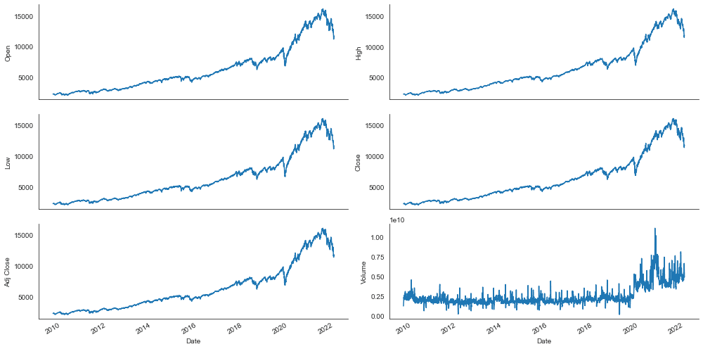
Our initial dataset includes six features: High, Low, Open, Close, Volumen, and Adj Close.
Step #3 Feature Engineering
Now comes the exciting part – we will implement additional features. We use various indicators from chart analysis, such as averages for different periods and stochastic oscillators to measure price momentum.
# Indexing Batches
train_df = df.sort_values(by=['Date']).copy()

# Adding Month and Year in separate columns
d = pd.to_datetime(train_df.index)
train_df['Day'] = d.strftime("%d")
train_df['Month'] = d.strftime("%m")
train_df['Year'] = d.strftime("%Y")
train_df
Open High Low Close Adj Close Volume Day Month Year Date 2009-12-31 2292.919922 2293.590088 2269.110107 2269.149902 2269.149902 1237820000 31 12 2009 2010-01-04 2294.409912 2311.149902 2294.409912 2308.419922 2308.419922 1931380000 04 01 2010 2010-01-05 2307.270020 2313.729980 2295.620117 2308.709961 2308.709961 2367860000 05 01 2010 2010-01-06 2307.709961 2314.070068 2295.679932 2301.090088 2301.090088 2253340000 06 01 2010 2010-01-07 2298.090088 2301.300049 2285.219971 2300.050049 2300.050049 2270050000 07 01 2010
We create a set of indicators for the training data with the following code. However, we will make one more restriction in the next step since a model with all these indicators does not achieve good results and would take far too long to train on a local computer.
# Feature Engineering
def createFeatures(df):
    df = pd.DataFrame(df)


    df['Close_Diff'] = df['Adj Close'].diff()

    # Moving averages - different periods
    df['MA200'] = df['Close'].rolling(window=200).mean()
    df['MA100'] = df['Close'].rolling(window=100).mean()
    df['MA50'] = df['Close'].rolling(window=50).mean()
    df['MA26'] = df['Close'].rolling(window=26).mean()
    df['MA20'] = df['Close'].rolling(window=20).mean()
    df['MA12'] = df['Close'].rolling(window=12).mean()

    # SMA Differences - different periods
    df['DIFF-MA200-MA50'] = df['MA200'] - df['MA50']
    df['DIFF-MA200-MA100'] = df['MA200'] - df['MA100']
    df['DIFF-MA200-CLOSE'] = df['MA200'] - df['Close']
    df['DIFF-MA100-CLOSE'] = df['MA100'] - df['Close']
    df['DIFF-MA50-CLOSE'] = df['MA50'] - df['Close']

    # Moving Averages on high, lows, and std - different periods
    df['MA200_low'] = df['Low'].rolling(window=200).min()
    df['MA14_low'] = df['Low'].rolling(window=14).min()
    df['MA200_high'] = df['High'].rolling(window=200).max()
    df['MA14_high'] = df['High'].rolling(window=14).max()
    df['MA20dSTD'] = df['Close'].rolling(window=20).std()

    # Exponential Moving Averages (EMAS) - different periods
    df['EMA12'] = df['Close'].ewm(span=12, adjust=False).mean()
    df['EMA20'] = df['Close'].ewm(span=20, adjust=False).mean()
    df['EMA26'] = df['Close'].ewm(span=26, adjust=False).mean()
    df['EMA100'] = df['Close'].ewm(span=100, adjust=False).mean()
    df['EMA200'] = df['Close'].ewm(span=200, adjust=False).mean()

    # Shifts (one day before and two days before)
    df['close_shift-1'] = df.shift(-1)['Close']
    df['close_shift-2'] = df.shift(-2)['Close']

    # Bollinger Bands
    df['Bollinger_Upper'] = df['MA20'] + (df['MA20dSTD'] * 2)
    df['Bollinger_Lower'] = df['MA20'] - (df['MA20dSTD'] * 2)

    # Relative Strength Index (RSI)
    df['K-ratio'] = 100*((df['Close'] - df['MA14_low']) / (df['MA14_high'] - df['MA14_low']) )
    df['RSI'] = df['K-ratio'].rolling(window=3).mean()

    # Moving Average Convergence/Divergence (MACD)
    df['MACD'] = df['EMA12'] - df['EMA26']

    # Replace nas
    nareplace = df.at[df.index.max(), 'Close']
    df.fillna((nareplace), inplace=True)

    return df
Now that we have created several features, we will limit them. We can now choose from these features and test how different feature combinations affect model performance.
# List of considered Features
FEATURES = [
#             'High',
#             'Low',
#             'Open',
              'Close',
#             'Volume',
#             'Day',
#             'Month',
#             'Year',
#             'Adj Close',
#              'close_shift-1',
#              'close_shift-2',
#             'MACD',
#             'RSI',
#             'MA200',
#             'MA200_high',
#             'MA200_low',
            'Bollinger_Upper',
            'Bollinger_Lower',
#             'MA100',
#             'MA50',
#             'MA26',
#             'MA14_low',
#             'MA14_high',
#             'MA12',
#             'EMA20',
#             'EMA100',
#             'EMA200',
#               'DIFF-MA200-MA50',
#               'DIFF-MA200-MA100',
#             'DIFF-MA200-CLOSE',
#             'DIFF-MA100-CLOSE',
#             'DIFF-MA50-CLOSE'
           ]

# Create the dataset with features
df_features = createFeatures(train_df)

# Shift the timeframe by 10 month
use_start_date = pd.to_datetime("2010-11-01" )
df_features = df_features[df_features.index > use_start_date].copy()

# Filter the data to the list of FEATURES
data_filtered_ext = df_features[FEATURES].copy()

# We add a prediction column and set dummy values to prepare the data for scaling
#data_filtered_ext['Prediction'] = data_filtered_ext['Close']
print(data_filtered_ext.tail().to_string())

# remove Date column before training
dfs = data_filtered_ext.copy()

# Create a list with the relevant columns
assetname_list = [dfs.columns[i-1] for i in range(dfs.shape[1])]

# Create the lineplot
fig, ax = plt.subplots(figsize=(16, 8))
sns.lineplot(data=data_filtered_ext[assetname_list], linewidth=1.0, dashes=False, palette='muted')

# Configure and show the plot
ax.set_title(stockname + ' price chart')
ax.legend()
plt.show
Close Bollinger_Upper Bollinger_Lower Date 2022-05-18 11418.150391 13404.779247 11065.040772 2022-05-19 11388.500000 13285.741255 11005.463725 2022-05-20 11354.620117 13214.664450 10928.073538 2022-05-23 11535.269531 13075.594634 10920.185347 2022-05-24 11264.450195 13035.543222 10837.607755 <function matplotlib.pyplot.show(close=None, block=None)>
Step #4 Scaling and Transforming the Data
Before training our model, we need to transform the data. This step includes scaling the data (to a range between 0 and 1) and dividing it into separate sets for training and testing the prediction model. Most of the code used in this section stems from the previous article on multivariate time-series prediction, which covers the steps to transform the data. So we don’t go into too much detail here.
# Calculate the number of rows in the data
nrows = dfs.shape[0]
np_data_unscaled = np.reshape(np.array(dfs), (nrows, -1))
print(np_data_unscaled.shape)

# Transform the data by scaling each feature to a range between 0 and 1
scaler = RobustScaler()
np_data = scaler.fit_transform(np_data_unscaled)

# Creating a separate scaler that works on a single column for scaling predictions
scaler_pred = RobustScaler()
df_Close = pd.DataFrame(data_filtered_ext['Close'])
np_Close_scaled = scaler_pred.fit_transform(df_Close)
Out: (2619, 6)
Once we have scaled the data, we will split the data into a train and test set. This step creates four datasets x_train and x_test, and y_train and y_test. x_train and x_test contain the data with our selected features. The two sets, y_train and y_test, have the actual values, which our model will try to predict.
# Set the sequence length - this is the timeframe used to make a single prediction
sequence_length = 50 # = number of neurons in the first layer of the neural network

# Split the training data into train and train data sets
# As a first step, we get the number of rows to train the model on 80% of the data
train_data_len = math.ceil(np_data.shape[0] * 0.8)

# Create the training and test data
train_data = np_data[:train_data_len, :]
test_data = np_data[train_data_len - sequence_length:, :]

# The RNN needs data with the format of [samples, time steps, features]
# Here, we create N samples, sequence_length time steps per sample, and 6 features
def partition_dataset(sequence_length, data):
    x, y = [], []
    data_len = data.shape[0]

    for i in range(sequence_length, data_len):
        x.append(data[i-sequence_length:i,:]) #contains sequence_length values 0-sequence_length * columsn
        y.append(data[i, 0]) #contains the prediction values for validation,  for single-step prediction

    # Convert the x and y to numpy arrays
    x = np.array(x)
    y = np.array(y)
    return x, y

# Generate training data and test data
x_train, y_train = partition_dataset(sequence_length, train_data)
x_test, y_test = partition_dataset(sequence_length, test_data)

# Print the shapes: the result is: (rows, training_sequence, features) (prediction value, )
print(x_train.shape, y_train.shape)
print(x_test.shape, y_test.shape)

# Validate that the prediction value and the input match up
# The last close price of the second input sample should equal the first prediction value
print(x_train[1][sequence_length-1][0])
print(y_train[0])
Out: (1914, 30, 3) (1914,) (486, 30, 3) (486,)
Step #5 Train the Time Series Forecasting Model
Now that we have prepared the data, we can train our forecasting model. For this purpose, we will use a recurrent neural network from the Keras library. A recurrent neural network (RNN) is a type of artificial neural network that can process sequential data, such as text, audio, or time series data. Unlike traditional feedforward neural networks, in which data flows through the network in only one direction, RNNs have connections that form a directed cycle, allowing information to flow in multiple directions and be processed in a temporal manner.
The model architecture of our RNN looks as follows:
- LSTM layer that receives a mini-batch as input.
- LSTM layer that has the same number of neurons as the mini-batch
- Another LSTM layer that does not return the sequence
- Dense layer with 32 neurons
- Dense layer with one neuron that outputs the forecast
The architecture is not too complex and is suitable for experimenting with different features. I arrived at this architecture by trying out different layers and configurations. However, I did not spend too much time fine-tuning the architecture since this tutorial focuses on feature engineering.
During model training, the neural network processes several mini-batches. The shape of the mini-batch is defined by the number of features and the period chosen. Multiplying these two dimensions (number of features x number of time steps) gives the input shape of our model.
The following code defines the model architecture, trains the model, and then prints the training loss curve:
# Configure the neural network model
model = Sequential()

# Configure the Neural Network Model with n Neurons - inputshape = t Timestamps x f Features
n_neurons = x_train.shape[1] * x_train.shape[2]
print('timesteps: ' + str(x_train.shape[1]) + ',' + ' features:' + str(x_train.shape[2]))
model.add(LSTM(n_neurons, return_sequences=True, input_shape=(x_train.shape[1], x_train.shape[2])))
#model.add(Dropout(0.1))
model.add(LSTM(n_neurons, return_sequences=True))
#model.add(Dropout(0.1))
model.add(LSTM(n_neurons, return_sequences=False))
model.add(Dense(32))
model.add(Dense(1, activation='relu'))


# Configure the Model
optimizer='adam'; loss='mean_squared_error'; epochs = 100; batch_size = 32; patience = 8;

# uncomment to customize the learning rate
learn_rate = "standard" # 0.05
# adam = Adam(learn_rate=learn_rate)

parameter_list = ['epochs ' + str(epochs), 'batch_size ' + str(batch_size), 'patience ' + str(patience), 'optimizer ' + str(optimizer) + ' with learn rate ' + str(learn_rate), 'loss ' + str(loss)]
print('Parameters: ' + str(parameter_list))

# Compile and Training the model
model.compile(optimizer=optimizer, loss=loss)
early_stop = EarlyStopping(monitor='loss', patience=patience, verbose=1)
history = model.fit(x_train, y_train, batch_size=batch_size, epochs=epochs, callbacks=[early_stop], shuffle = True,
                  validation_data=(x_test, y_test))

# Plot training & validation loss values
fig, ax = plt.subplots(figsize=(12, 6), sharex=True)
plt.plot(history.history["loss"])
plt.title("Model loss")
plt.ylabel("Loss")
plt.xlabel("Epoch")
ax.xaxis.set_major_locator(plt.MaxNLocator(epochs))
plt.legend(["Train", "Test"], loc="upper left")
plt.show()
timesteps: 50, features:1 Parameters: ['epochs 100', 'batch_size 32', 'patience 8', 'optimizer adam with learn rate standard', 'loss mean_squared_error'] Epoch 1/100 72/72 [==============================] - 9s 55ms/step - loss: 0.0990 - val_loss: 0.2985 Epoch 2/100 72/72 [==============================] - 3s 37ms/step - loss: 0.0932 - val_loss: 0.1768 Epoch 3/100 72/72 [==============================] - 3s 39ms/step - loss: 0.0931 - val_loss: 0.1246 Epoch 4/100 72/72 [==============================] - 3s 37ms/step - loss: 0.0931 - val_loss: 0.0902 Epoch 5/100 72/72 [==============================] - 3s 38ms/step - loss: 0.0929 - val_loss: 0.0846 Epoch 6/100 72/72 [==============================] - 3s 38ms/step - loss: 0.0930 - val_loss: 0.0611 Epoch 7/100 72/72 [==============================] - 3s 38ms/step - loss: 0.0929 - val_loss: 0.0498 Epoch 8/100 72/72 [==============================] - 3s 37ms/step - loss: 0.0928 - val_loss: 0.0208 Epoch 9/100 72/72 [==============================] - 3s 38ms/step - loss: 0.0929 - val_loss: 0.0588 Epoch 10/100 72/72 [==============================] - 3s 37ms/step - loss: 0.0928 - val_loss: 0.0437 Epoch 11/100 72/72 [==============================] - 3s 36ms/step - loss: 0.0928 - val_loss: 0.0192 Epoch 12/100 ... 72/72 [==============================] - 3s 38ms/step - loss: 0.0925 - val_loss: 0.0094 Epoch 46/100 72/72 [==============================] - 3s 37ms/step - loss: 0.0925 - val_loss: 0.0113 Epoch 00046: early stopping
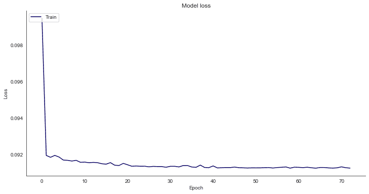
The loss drops quickly, and the training process looks promising.
Step #6 Evaluate Model Performance
If we test a feature, we also want to know how it impacts the performance of our model. Feature Engineering is therefore closely related to evaluating model performance. So, let’s check the prediction performance. For this purpose, we score the model with the test data set (x_test). Then we can compare the predictions with the actual values (y_test) in a lineplot.
# Get the predicted values
y_pred_scaled = model.predict(x_test)

# Unscale the predicted values
y_pred = scaler_pred.inverse_transform(y_pred_scaled)
y_test_unscaled = scaler_pred.inverse_transform(y_test.reshape(-1, 1))
y_test_unscaled.shape

# Mean Absolute Error (MAE)
MAE = mean_absolute_error(y_test_unscaled, y_pred)
print(f'Median Absolute Error (MAE): {np.round(MAE, 2)}')

# Mean Absolute Percentage Error (MAPE)
MAPE = np.mean((np.abs(np.subtract(y_test_unscaled, y_pred)/ y_test_unscaled))) * 100
print(f'Mean Absolute Percentage Error (MAPE): {np.round(MAPE, 2)} %')

# Median Absolute Percentage Error (MDAPE)
MDAPE = np.median((np.abs(np.subtract(y_test_unscaled, y_pred)/ y_test_unscaled)) ) * 100
print(f'Median Absolute Percentage Error (MDAPE): {np.round(MDAPE, 2)} %')

# The date from which on the date is displayed
display_start_date = "2019-01-01"

# Add the difference between the valid and predicted prices
train = pd.DataFrame(dfs['Close'][:train_data_len + 1]).rename(columns={'Close': 'y_train'})
valid = pd.DataFrame(dfs['Close'][train_data_len:]).rename(columns={'Close': 'y_test'})
valid.insert(1, "y_pred", y_pred, True)
valid.insert(1, "residuals", valid["y_pred"] - valid["y_test"], True)
df_union = pd.concat([train, valid])

# Zoom in to a closer timeframe
df_union_zoom = df_union[df_union.index > display_start_date]

# Create the lineplot
fig, ax1 = plt.subplots(figsize=(16, 8))
plt.title("y_pred vs y_test")
plt.ylabel(stockname, fontsize=18)
sns.set_palette(["#090364", "#1960EF", "#EF5919"])
sns.lineplot(data=df_union_zoom[['y_pred', 'y_train', 'y_test']], linewidth=1.0, dashes=False, ax=ax1)

# Create the barplot for the absolute errors
df_sub = ["#2BC97A" if x > 0 else "#C92B2B" for x in df_union_zoom["residuals"].dropna()]
ax1.bar(height=df_union_zoom['residuals'].dropna(), x=df_union_zoom['residuals'].dropna().index, width=3, label='absolute errors', color=df_sub)
plt.legend()
plt.show()
Median Absolute Error (MAE): 547.23 Mean Absolute Percentage Error (MAPE): 4.04 % Median Absolute Percentage Error (MDAPE): 3.73 %

On average, the predictions of our model deviate from the actual values by about one percent. Although one percent may not sound like a lot, the prediction errors can quickly accumulate to larger values.
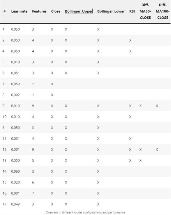
Step #7 Overview of Selected Models
In writing this article, I tested various models based on different features. The neural network architecture remained unchanged. Likewise, I kept the hyperparameters the same except for the learning rate. Below are the results of these model variants:
Step #8 Conclusions
Estimating which indicators will lead to good results in advance is difficult. More indicators do not necessarily lead to better results because they increase the model complexity and add data without predictive power. This so-called noise makes it harder for the model to separate important influencing factors from less important ones. Also, each additional indicator increases the time needed to train the model. So there is no way around testing different variants.
Besides the feature, various hyperparameters such as the learning rate, optimizer, batch size, and the selected time frame of the data (sequence_length) impact the model’s performance. Tuning these hyperparameters can further improve model performance.
- A learning rate of 0.05 achieves the best results from the tested configurations.
- Of all features, only the Bollinger bands positively affected the model’s performance.
- As expected, the performance tends to decrease with the number of features.
- In our case, the hyperparameters seem to affect the performance of the models more than the choice of features.
Finally, we have optimized only a single parameter. We searched for optimal learning rates while leaving all other parameters unchanged, such as the optimizer, the neural network architecture, or the sequence length. Based on the results, we can draw several conclusions:
There is plenty of room for improvement and experimentation. With more time for experiments and computational power, it will undoubtedly be possible to identify better features and model configurations. So, have fun experimenting! 🙂
Summary
In this tutorial, we have delved into the fascinating world of feature engineering for stock market forecasting using Python. By exploring various features from chart analysis, such as RSI, moving averages, and Bollinger bands, we have developed multiple variants of a recurrent neural network that produce distinct prediction models.
Our experiments have shown that the choice of features can have a significant impact on the performance of the prediction model. Therefore, it’s essential to carefully select features and consider their potential impact on the model. Additionally, keep in mind that the most effective features for recognizing patterns in historical data will vary depending on the specific time series data being analyzed.
By following the crucial steps outlined in this tutorial, you now have the knowledge and tools to apply feature engineering techniques to any multivariate time series forecasting problem. With further experimentation and testing, you can fine-tune your models to achieve the best possible results for your specific use case.
We hope you found this tutorial both informative and helpful. If you have any questions or comments, don’t hesitate to reach out and let us know.
And if you want to learn more about feature preparation and exploration, check out my recent article on Exploratory Feature Preparation for Regression Models.
Sources and Further Reading
- Charu C. Aggarwal (2018) Neural Networks and Deep Learning
- Jansen (2020) Machine Learning for Algorithmic Trading: Predictive models to extract signals from market and alternative data for systematic trading strategies with Python
- Aurélien Géron (2019) Hands-On Machine Learning with Scikit-Learn, Keras, and TensorFlow: Concepts, Tools, and Techniques to Build Intelligent Systems
- David Forsyth (2019) Applied Machine Learning Springer
- Andriy Burkov (2020) Machine Learning Engineering
The links above to Amazon are affiliate links. By buying through these links, you support the Relataly.com blog and help to cover the hosting costs. Using the links does not affect the price.
Books on Applied Machine Learning
The links above to Amazon are affiliate links. By buying through these links, you support the Relataly.com blog and help to cover the hosting costs. Using the links does not affect the price.

Hi Florian
Thank you for sharing this valuable work. This led me to better understand predictive models (I’m a newbie) and concrete examples of how to exploit them. So I started playing around and I found a strange behaviour where y_pred gets a constant value when I use your configuration with different stocknames such as ISP.MI, BPE.MI and many others. I tried to investigate, with my limited capabilities, and I discovered that the “model.predict(x_test) command returns some 0 values.
Here an example
Hello Florian,
There is an error in your code, you print your features but you DON’T use them in your model.
# Create the training and test data
train_data = np_Close_scaled[:train_data_len, :]
test_data = np_Close_scaled[train_data_len – sequence_length:, :]
Your model only use your Close as Label/Features, you should use :
train_data = dfs[:train_data_len, :]
test_data = dfs[train_data_len – sequence_length:, :]
with your Close in 1st Column of dfs to suit your code.
Thank you for your posts btw, they are very helpfull.
Hello Mat,
Thank you for bringing this to my attention! This was indeed a mistake.
Best,
Florian
Hi,
I understood this. Can u explain how we can proceed with this feature engineering for solar power forecasting? How can we consider the new features for modeling?
Thanks for the interesting question! Some statistical indicators from stock market prediction, such as moving averages, standard deviations, and trend lines, may also be useful in analyzing solar power data. For example, a moving average could be used to smooth out fluctuations in solar power generation data, making it easier to identify underlying trends. Similarly, a trend line could be used to identify long-term patterns in solar power generation data.
However, ithe factors that influence stock market movements and solar power generation are quite different. So the statistical indicators that are effective in stock market prediction e.g., bollinger bands, RSI, etc. may not be as effective.
Hope this helps, best
Florian
Hello.
I tried to run your code, but running it gives me the following error:
# Shift the timeframe by 10 month
use_start_date = pd.to_datetime(“2010-11-01” )
data = data[data[‘Date’] > use_start_date].copy()
Error:
KeyError: ‘Date’
I appreciate your support
Hi Jose, thanks for letting me know. Indeed, there was an error in the code. I fixed it and the code should work now.