Stock Market Prediction using Univariate Recurrent Neural Networks (RNN) with Python

Financial analysts have long been fascinated by the prospect of predicting the prices of financial assets. In recent years, there has been increasing interest in using machine learning and deep learning techniques to generate predictions, in addition to traditional methods such as technical and fundamental analysis. Python libraries like Keras and Scikit-Learn make it relatively straightforward for those with programming experience to build a neural network for stock market forecasting. This tutorial will guide you through the process of creating a univariate model using a Keras neural network with LSTM layers to forecast the S&P500 index. By the end of this tutorial, you will have a model that can make single-step predictions for the stock market.

The rest of this article proceeds in two parts: We briefly introduce univariate modeling and neural networks. Then we start with the coding part and go through all the steps to train a neural network, including data ingestion, data preprocessing, and the design, training, testing, and usage of a predictive neural network model.

Disclaimer

This article does not constitute financial advice. Stock markets can be very volatile and are generally difficult to predict. Predictive models and other forms of analytics applied in this article only serve the purpose of illustrating machine learning use cases.

AI can help investors and traders to make more accurate investment decisions.

Single-Step Univariate Stock Market Prediction

The prediction approach described in this article is known as single-step single-variate time series forecasting. This approach is similar to technical chart analysis in that it assumes that predicting the price of an asset is fundamentally a time series problem. The goal is to identify patterns in a time series that indicate how the series will develop in the future.

This tutorial predicts the value for a single time step (1 day). In other words, we consider a single time series of data (single-variate). However, predicting multiple steps or increasing the time-step length would also be possible. In both cases, the predictions will range further into the future. I have covered this topic in a separate post on time series forecasting.

We will develop a univariate prediction model that predicts a single feature on historical prices for a specific period. More complex multivariate models use additional features such as moving averages, momentum indicators, or market sentiment. I have covered multivariate stock market prediction in a separate tutorial.

What are Recurrent Neural Networks?

Recurrent Neural Networks (RNNs) process sequences by carrying a hidden state from one time step to the next. LSTM is one type of recurrent layer. Its gates help retain and discard information over longer sequences, reducing some of the vanishing-gradient problems found in simple RNNs. A standard LSTM processes the sequence in chronological order; information only flows in both directions when a bidirectional architecture is used.

One of the primary advantages of RNNs is their ability to process sequential data, such as time series or natural language text. This is because the LSTM layers in an RNN allow the network to maintain a sense of memory and context, allowing it to understand the relationships between data points better and make more accurate predictions.

RNNs are commonly used in a wide range of applications, including language translation, speech recognition, and sentiment analysis. In these applications, the input data is often a sequence of words or other elements. The RNN can use its memory and context-aware processing to understand the meaning and relationships between the elements in the sequence.

Inspired by nature: Each layer of neurons extracts different features from the input data, and the output of one layer becomes the input for the next layer until the final output is generated.

Also: Stock Market Forecasting Neural Networks for Multi-Output Regression in Python

Creating a Univariate Forecasting Model using Keras Recurrent Neural Networks in Python

In this article, we will showcase the process of building a univariate forecast for the closing price of the S&P500 stock market index. To achieve this, we will use a Recurrent Neural Network (RNN) architecture with Long Short-Term Memory (LSTM) layers based on the popular Tensorflow library. In addition, we will employ various Python packages for data manipulation and analytics. The process of training and using the univariate model involves several key steps:

1. Loading the data
2. Exploring the data to identify trends and patterns
3. Scaling and splitting the data to prepare it for modeling
4. Creating the input shape to feed the data into the LSTM network
5. Training the model on the training data set
6. Forecasting future values using the trained model
7. Visualizing and interpreting the forecasted results

By following these steps, we will create an illustrative one-step forecast for the S&P 500 closing value and test whether it improves on a simple persistence forecast. The baseline comparison is essential: a neural network is only useful if it adds predictive value beyond assuming that the next close equals the latest close.

The Python code is available in the relataly GitHub repository.

Please note that you will need some programming experience and familiarity with Python to follow along with this article. Understanding Neural Networks in all depth is not a prerequisite for this tutorial. But if you want to learn more about their architecture and functioning, I can recommend this YouTube video.

Prerequisites

Before starting the coding part, make sure that you have set up your Python 3 environment and required packages. If you don’t have an environment yet, you can follow the steps in this article to set up the Anaconda environment. Also, make sure you install all required packages. In this tutorial, we will be working with the following standard packages:

• pandas
• NumPy
• matplotlib

In addition, we will use Keras 3 with the TensorFlow backend, scikit-learn, seaborn, and yfinance. The refreshed notebook was tested with Python 3.12, TensorFlow 2.21, Keras 3.15, pandas 3.0, scikit-learn 1.9, and yfinance 1.5.

You can install packages using console commands:

• pip install
• conda install  (if you are using the anaconda packet manager)

Step #1 Load the Data

Let’s start by setting up the imports and loading price data from Yahoo Finance with yfinance. Current yfinance versions return MultiIndex columns by default, even for one ticker. We set multi_level_index=False explicitly so later code receives ordinary Close, High, Low, Open, and Volume columns.

The following code extracts S&P 500 data from 2010 through the end of 2025. ^GSPC is Yahoo Finance’s symbol for the index. You can replace it with another symbol, such as BTC-USD for Bitcoin. A fixed endpoint makes the train/test split and reported metrics reproducible. We also set auto_adjust=True explicitly, matching yfinance’s current default.

# A tutorial for this file is available at www.relataly.com
# Tested with Python 3.12, TensorFlow 2.21, Keras 3.15, pandas 3.0, and yfinance 1.5

import keras
import matplotlib.dates as mdates
import matplotlib.pyplot as plt
import numpy as np
import pandas as pd
import seaborn as sns
import tensorflow as tf
import yfinance as yf
from sklearn.metrics import mean_absolute_error, root_mean_squared_error
from sklearn.preprocessing import MinMaxScaler

sns.set_theme(style="white", rc={"axes.spines.right": False, "axes.spines.top": False})
keras.utils.set_random_seed(42)

print(f"TensorFlow version: {tf.__version__}")
print(f"Available GPUs: {len(tf.config.list_physical_devices('GPU'))}")

# Use a fixed, recent endpoint so the tutorial produces reproducible train/test sets.
start_date = "2010-01-01"
end_date = "2026-01-01"
stock_name = "S&P 500"
symbol = "^GSPC"

df = yf.download(
  symbol,
  start=start_date,
  end=end_date,
  auto_adjust=True,
  multi_level_index=False,
  progress=False,
)
if df.empty:
  raise RuntimeError("yfinance returned no data for ^GSPC")

print(df.shape)
df.head()

TensorFlow version: 2.21.0
Available GPUs: 0
(4024, 5)

The GPU count depends on your environment. TensorFlow 2.11 and newer do not support native-Windows NVIDIA GPU acceleration; use WSL2 for that setup. CPU execution works for this tutorial.

Step #2 Explore the Data

When you load a new data set into your project, it is often a good idea to familiarize yourself with it before taking further steps. When working with time-series data, visually viewing the data in a line plot is the primary way. Use the following code to create the line plot for the S&P500 data.

years = mdates.YearLocator()
_, ax = plt.subplots(figsize=(16, 6))
ax.xaxis.set_major_locator(years)
sns.lineplot(x=df.index, y=df["Close"], ax=ax, label=stock_name, linewidth=1.0)
ax.set_title(f"{stock_name} from {start_date} to {end_date}")
ax.set_ylabel("Index points")
ax.legend(fontsize=12)
plt.show()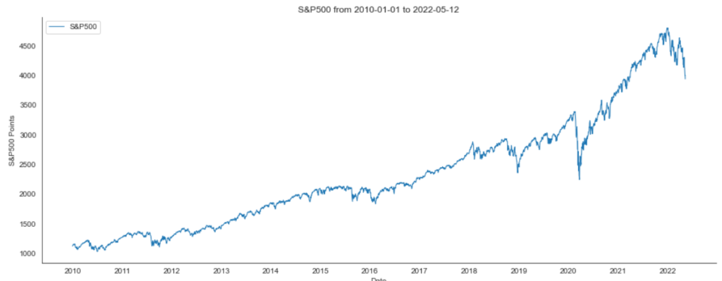

If you follow the course of the S&P500 stock markets a little, the chart above might look familiar to you.

Step #3 Scaling the Data

It’s best to scale the data before training a neural network. We use MinMaxScaler, but fit it only on the training period. Fitting preprocessing on the complete series would leak the future test-set price range into model development. Test values may fall outside the nominal 0-to-1 training range, which is valid and preferable to leakage.

close_prices = df[["Close"]].dropna().copy()
train_size = int(len(close_prices) * 0.8)

# Fit preprocessing on the training period only to avoid leaking future price ranges.
scaler = MinMaxScaler(feature_range=(0, 1))
scaler.fit(close_prices.iloc[:train_size])
scaled_prices = scaler.transform(close_prices)

Step #4 Creating the Input Shape

Before we can begin with the training of the NN, we need to split the data into separate test sets for training and validation and ensure that it is in the right shape. We will train the NN on a decade of market price data. Then we predict the price of the next day based on the last 50 days of market prices. As illustrated below, we will use 80% of the data as training data and keep 20% as test data to later evaluate the performance of our univariate model.

Splitting data into train and test

Our neural network will have two layers, an input layer, and an output layer. The input data shape must correspond with the number of neurons in the neural network’s input layer. Therefore, we must also decide on the neural network architecture before bringing our data in the right shape.

4.1 Designing the Input Shape

Next, we create the training data based on which we will train our neural network. We make multiple slices of the training data (x_train), so-called mini-batches. The neural network processes the mini-batch one by one during the training process and creates a separate forecast for each mini-batch. The illustration below shows the shape of the data:

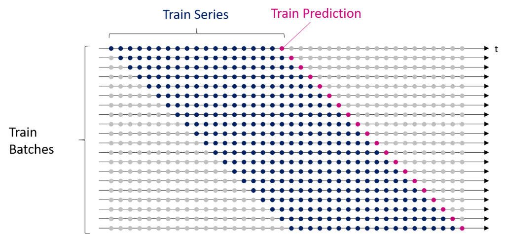
The sample dataset for time series forecasting is split into several train batches.

Neural networks learn in an iterative process. The algorithm reduces the prediction errors by adjusting the connection strength between the neurons (weights) in this process. The model needs a second list (y_train) to evaluate the forecast quality, containing the valid price values from our ground truth. The model compares the predictions with the ground truth during training and calculates the training error to minimize it over time.

4.2 Data Preprocessing

The code below creates overlapping samples. Each sample contains 50 closing values and one target: the following close. We prepend the final 50 training observations to the test slice so the first held-out prediction has a complete history without discarding test dates.

sequence_length = 50


def create_sequences(values, sequence_length):
  features, targets = [], []
  for index in range(sequence_length, len(values)):
    features.append(values[index - sequence_length:index])
    targets.append(values[index, 0])

  return (
    np.asarray(features, dtype=np.float32),
    np.asarray(targets, dtype=np.float32),
  )


train_values = scaled_prices[:train_size]
test_values = scaled_prices[train_size - sequence_length:]
x_train, y_train = create_sequences(train_values, sequence_length)
x_test, y_test = create_sequences(test_values, sequence_length)

print(f"Training shapes: {x_train.shape}, {y_train.shape}")
print(f"Test shapes: {x_test.shape}, {y_test.shape}")

# The first test target follows the final 50 observations ending at the split.
assert np.isclose(x_test[0, -1, 0], scaled_prices[train_size - 1, 0])
assert np.isclose(y_test[0], scaled_prices[train_size, 0])

Training shapes: (3169, 50, 1), (3169,)
Test shapes: (805, 50, 1), (805,)

x_train contains 3,169 samples. Each has 50 time steps and one feature. y_train contains one next-day target per sample. These shapes remain stable because the data endpoint is fixed.

Step #5 Designing the Model Architecture

Before we can train the model, we first need to decide on the model’s architecture. Above all, the architecture comprises the type and number of layers and the number of neurons in each layer.

5.1 Choosing Layers

Determining the optimal number of layers for a neural network can be challenging and often requires trial and error. One approach is to try out different architectures and see which one performs best. In this case, we will use a fully connected network with four layers, consisting of two layers of the LSTM class and two layers of the Dense class from the Keras library. This architecture was chosen because it is relatively simple and a good starting point for addressing time series problems. The architecture and performance of the univariate model can then be tested and refined through multiple iterations.

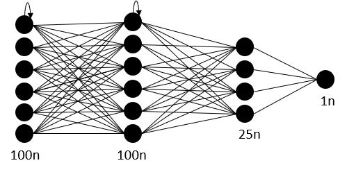
The architecture of our recurrent Neural Network

5.2 Choosing the Number of Neurons

When selecting the number of neurons for a neural network layer, there are a few general guidelines to follow:

• A larger number of neurons can allow the model to capture more complex patterns in the data, but it may also increase the risk of overfitting.
• A smaller number of neurons can reduce the risk of overfitting, but it may also limit the model’s ability to capture complex patterns.
• It is generally recommended to start with a smaller number of neurons and increase the number if necessary.

The sequence length and the number of LSTM units are different choices. Our input has 50 time steps and one feature per time step; this does not require at least 50 recurrent units. The number of units controls model capacity and should be tuned with chronological validation. We use 50 units in each LSTM layer and 25 units in the dense hidden layer as a compact teaching architecture. The final layer has one unit because we predict one value.

model = keras.Sequential(
  [
    keras.layers.Input(shape=(sequence_length, 1)),
    keras.layers.LSTM(50, return_sequences=True),
    keras.layers.LSTM(50),
    keras.layers.Dense(25, activation="relu"),
    keras.layers.Dense(1),
  ],
  name="sp500_lstm",
)
model.compile(optimizer=keras.optimizers.Adam(), loss="mean_squared_error")
model.summary()

Step #6 Train the Univariate Model

Now that we have prepared the data and defined the model, we fit it on the training samples. The final 10% of the training samples becomes a chronological validation segment. We disable shuffling, stop after three epochs without validation improvement, and restore the best weights. The untouched 20% test period remains unavailable to model selection.

early_stopping = keras.callbacks.EarlyStopping(
  monitor="val_loss",
  patience=3,
  restore_best_weights=True,
)
history = model.fit(
  x_train,
  y_train,
  batch_size=32,
  epochs=20,
  validation_split=0.1,
  shuffle=False,
  callbacks=[early_stopping],
  verbose=1,
)

Epoch 16/20
90/90 - loss: 2.5026e-04 - val_loss: 0.0013

On the tested run, early stopping ends training after epoch 16 and restores the weights from the best validation epoch.

Step #7 Creating the Univariate Stock Market Forecasting

So how does our stock market prediction model perform? We need to feed the model with the test data to evaluate the model’s performance. For this purpose, we provide the test data (x_test) that we have generated in a previous step to the model to get some predictions. We must remember that we initially scaled the input data to 0 and 1. Therefore, before interpreting the results, we must inverse the MinMaxScaling from the predictions.

y_pred_scaled = model.predict(x_test, verbose=0)
y_pred = scaler.inverse_transform(y_pred_scaled).ravel()
y_test_unscaled = scaler.inverse_transform(y_test.reshape(-1, 1)).ravel()

Step #8 Evaluate Model Performance

Different indicators help us evaluate the model. MAE and RMSE are always non-negative because they summarize absolute or squared errors. We also report percentage errors and compare the neural network with a persistence baseline that uses the latest observed close as the next prediction.

absolute_percentage_errors = np.abs((y_test_unscaled - y_pred) / y_test_unscaled) * 100
mae = mean_absolute_error(y_test_unscaled, y_pred)
rmse = root_mean_squared_error(y_test_unscaled, y_pred)
mape = absolute_percentage_errors.mean()
median_ape = np.median(absolute_percentage_errors)

# A one-step persistence forecast predicts that tomorrow closes at today's value.
naive_pred = close_prices["Close"].iloc[train_size - 1:-1].to_numpy()
naive_mae = mean_absolute_error(y_test_unscaled, naive_pred)
naive_rmse = root_mean_squared_error(y_test_unscaled, naive_pred)

print(f"LSTM MAE: {mae:.2f} index points")
print(f"LSTM RMSE: {rmse:.2f} index points")
print(f"LSTM MAPE: {mape:.2f}%")
print(f"LSTM median absolute percentage error: {median_ape:.2f}%")
print(f"Persistence baseline MAE: {naive_mae:.2f} index points")
print(f"Persistence baseline RMSE: {naive_rmse:.2f} index points")

LSTM MAE: 237.18 index points
LSTM RMSE: 309.49 index points
LSTM MAPE: 4.14%
LSTM median absolute percentage error: 3.63%
Persistence baseline MAE: 35.17 index points
Persistence baseline RMSE: 50.65 index points

The LSTM does not beat persistence on this held-out period. Its MAE is about 6.7 times larger, and its RMSE is about 6.1 times larger. The raw-price model increasingly lags the rising index level. This result is a useful reminder that model complexity does not guarantee predictive value. Further work could model returns, add explanatory features, tune the architecture, and use rolling-origin evaluation, but every candidate should still be compared with simple baselines.

Visualizing test predictions helps in the process of evaluating the model. Therefore we will plot predicted and valid values.

test_index = close_prices.index[train_size:]
evaluation = pd.DataFrame(
  {
    "Actual": y_test_unscaled,
    "LSTM": y_pred,
    "Persistence baseline": naive_pred,
  },
  index=test_index,
)
evaluation["LSTM residual"] = evaluation["LSTM"] - evaluation["Actual"]

_, (ax_price, ax_error) = plt.subplots(
  2,
  1,
  figsize=(16, 9),
  sharex=True,
  gridspec_kw={"height_ratios": [3, 1]},
)
sns.lineplot(data=evaluation[["Actual", "LSTM", "Persistence baseline"]], ax=ax_price)
ax_price.set_title("Held-Out Predictions vs. Ground Truth")
ax_price.set_ylabel("S&P 500 index points")

colors = np.where(evaluation["LSTM residual"] >= 0, "#2B8A3E", "#C92A2A")
ax_error.bar(evaluation.index, evaluation["LSTM residual"], width=3, color=colors)
ax_error.axhline(0, color="black", linewidth=1)
ax_error.set_ylabel("LSTM residual")
plt.tight_layout()
plt.show()

The upper panel shows that persistence nearly overlaps the actual series, while the LSTM drifts below it. The lower panel shows signed LSTM residuals, defined as prediction minus actual. Negative bars mean that the model underpredicted.

Step #9 Stock Market Prediction - Predicting a Single Day Ahead

We can still demonstrate the mechanics of a single next-session prediction with the final 50 observations. Because the held-out evaluation is poor, this output is illustrative and should not be used for a trading decision.

last_sequence_scaled = scaler.transform(close_prices.iloc[-sequence_length:])
x_next = last_sequence_scaled[np.newaxis, ...].astype(np.float32)
next_close_scaled = model.predict(x_next, verbose=0)
next_close = float(scaler.inverse_transform(next_close_scaled)[0, 0])

last_date = close_prices.index[-1].date()
last_close = float(close_prices["Close"].iloc[-1])
percent_change = (next_close / last_close - 1) * 100

print(f"Last observed {stock_name} close on {last_date}: {last_close:.2f}")
print(f"Illustrative next-session prediction: {next_close:.2f} ({percent_change:+.2f}%)")

Last observed S&P 500 close on 2025-12-31: 6845.50
Illustrative next-session prediction: 6190.69 (-9.57%)

The large predicted drop is inconsistent with the model’s weak held-out performance and should be read as another warning about relying on this specification.

Summary

In this tutorial, you learned to create, train, and test a four-layer recurrent neural network for one-step stock-index prediction with Python and Keras. The refresh also demonstrated three practices that materially affect the conclusion: fit preprocessing only on training data, preserve chronological validation, and compare the result with a simple baseline.

On the 2022-2025 held-out period, this LSTM underperforms persistence by a wide margin. It remains useful as a compact example of the sequence-modeling workflow, while its forecasts should not be treated as evidence of a tradable signal. Replacing the symbol is easy; building a model that generalizes requires fresh evaluation and stronger features or targets.

The model created in this post makes predictions for a single time step. If you want to learn how to make time-series predictions that range further, you might want to check out the part II of this tutorial series: Creating a Multistep Forecast in Python.

I hope you enjoyed this article. I am always trying to improve and learn from my audience. So, please let me know in the comments if you have questions or remarks!

The Bulls and the Bears - a never-ending struggle but in the long run, the bulls tend to win. Image created with Midjourney.

Sources and Further Reading

1. Charu C. Aggarwal (2018) Neural Networks and Deep Learning
2. Jansen (2020) Machine Learning for Algorithmic Trading: Predictive models to extract signals from market and alternative data for systematic trading strategies with Python
3. Aurélien Géron (2019) Hands-On Machine Learning with Scikit-Learn, Keras, and TensorFlow: Concepts, Tools, and Techniques to Build Intelligent Systems
4. David Forsyth (2019) Applied Machine Learning Springer
5. Andriy Burkov (2020) Machine Learning Engineering
6. ChatGPT helped to revise this article.
7. Images created with Midjourney.

The links above to Amazon are affiliate links. By buying through these links, you support the Relataly.com blog and help to cover the hosting costs. Using the links does not affect the price.

If you want to learn about an alternative approach to univariate stock market forecasting, consider this article on Facebook Prophet.