Build a High-Performing Movie Recommender System using Collaborative Filtering in Python

An Overview of Recommender Techniques

The first attempts with recommendation systems reach back to the 1970s. The approach was relatively simple and categorized users into groups to suggest the same content to all users in the same group. However, it was a breakthrough because, for the first time, a program could make personalized recommendations. As the importance of recommendation engines increased, so did the interest in improving their predictions.

With the rise of the internet and the rapidly growing amount of data available on the web, filtering relevant content has become increasingly important. Large tech companies such as Netflix (TV shows and movies), Amazon (products), or Facebook (user content and profiles) understood early on that they could use recommendation systems to personalize the selection of user content shown to their customers. They all face the same challenge of having massive content and only limited space to display it to their users. Therefore, it has become crucial for them to select and display only the content that matches the individual interests of their users.

Internet companies are predestined for using recommender systems, as they have massive amounts of user data available. The user data is the foundation for generating personalized recommendations on a large scale by analyzing behavior patterns among larger groups of users to tailor suggestions to the taste of individuals.

Three Common Approaches to Recommender Systems

Nowadays, many different approaches can generate recommendations. However, most recommender systems use one of the following three techniques:

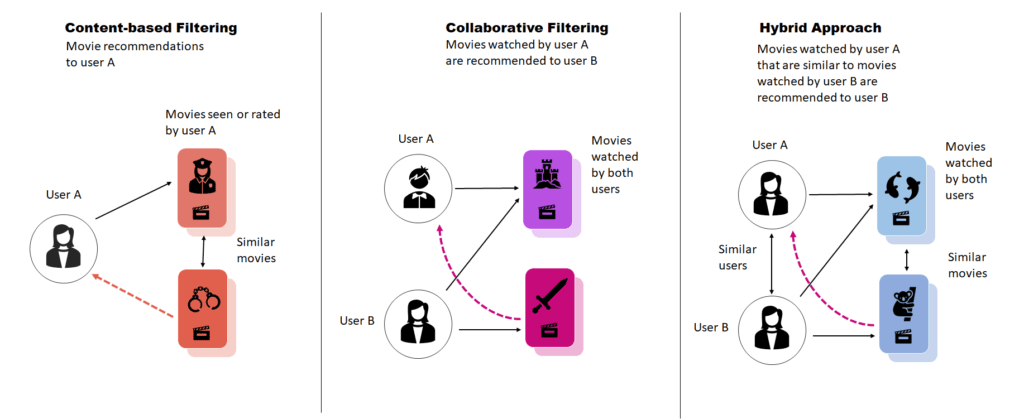
Content-based Filtering 

Content-based filtering is a technique that recommends similar items based on item content. Naturally, this approach is based on metadata to determine which items are similar. For example, in the case of movie recommendations, the algorithm would look at the genre, cast, or director of a movie. Models may also consider metadata on users, such as age, gender, etc., to suggest similar content to similar users. There are different methods to calculate the similarity, for example, Cosine Similarity or Minkowski Distance.

A significant challenge in content-based Filtering is the transferability of user preference insights from one item type to another. Often, content-based recommenders struggle to transfer user actions on one item (e.g., book) to other content types (e.g., clothing). In addition, content-based systems tend to develop tunnel vision, leading the engine to recommend more and more of the same.

A separate article covers content-based filtering in more detail and shows how to implement this approach for movie recommendations.

Collaborative Filtering

Collaborative Filtering is a well-established approach used to build recommendation systems. The recommendations generated through Collaborative Filtering are based on past interactions between a user and a set of items (movies, products, etc.) that are matched against past item-user interactions within a larger group of people. The main idea is to use the interactions between a group of users and a group of items to guess how users rate items they have not yet rated before.

A challenge of collaborative filters is known as the cold start problem, which refers to the entry of new users into the system without any ratings. As a result, the engine does not know its interests and cannot make meaningful recommendations. The same applies to new items entering the system (e.g., products) that have not yet received any ratings. As a result, recommendations can become self-reinforcing. Popular content that many users have rated is recommended to almost all other users, making this content even more popular. On the other hand, the engine hardly suggests content with few or no ratings, so no one will rate this content.

Hybrid Approach

Combining the previous two techniques in a hybrid approach is also possible. We can implement hybrid approaches by generating content-based and collaborative-based predictions separately and then combining them. The result is a model that considers the interactions between users and items and context information. Hybrid recommender systems often achieve better results than recommendation approaches that use a single of the underlying techniques.

Netflix is known to use a hybrid recommendation system. Its engine recommends content to its users based on similar users’ viewing and search habits (Collaborative Filtering). At the same time, it also recommends series and movies whose characteristics match the content users rated highly (content-based Filtering).

How Model-based Collaborative Filtering Works

We can further differentiate between memory-based and model-based Collaborative Filtering. This tutorial focuses on model-based Collaborative Filtering, which is more commonly used.

Behavioral Patterns: Dependencies among Users and Items

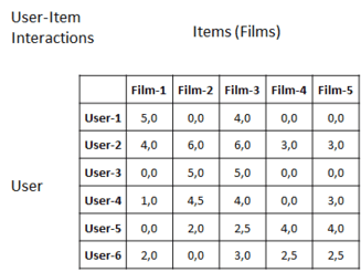
Collaborative filtering searches for behavioral patterns in interactions between a group of users and a group of items to infer the interests of individuals. The input data for collaborative Filtering is typically in the form of a user/item matrix filled with ratings (as shown below).

Patterns can exist in the user/item matrix in dependencies between users and items. Some dependencies are easy to grasp. Similar dependencies exist between items in that some movies receive high ratings from the same users. For example, assume two users, Ron and Joe, have rated movies. Ron enjoyed Batman, Indiana Jones, Star Wars, and Godzilla. Joe enjoyed the same movies as Ron, except Godzilla, which he has not yet rated. Based on the similarity between Joe and Ron, we assume that Joe would also enjoy Godzilla.

Things get more complex as latent dependencies are present in the data. Imagine Bob gave a three-star rating to five different movies. Another user, Jenny, rated the same movies as Bob but always gave four stars, which is an example of latent dependency. There is some form of dependence between the two users, and although it is not as significant as in the first example, considering latent dependencies will improve predictions.

Machine Learning and Dimensionality Reduction

Model-based collaborative filtering techniques estimate the parameters of statistical models to predict how individual users would rate an unrated item. A widely used approach formulates this problem as a classification task that considers items over users as features and ratings as prediction labels (as shown in the matrix). We can use various algorithms to solve such an optimization problem, including gradient-based techniques or alternating least squares.

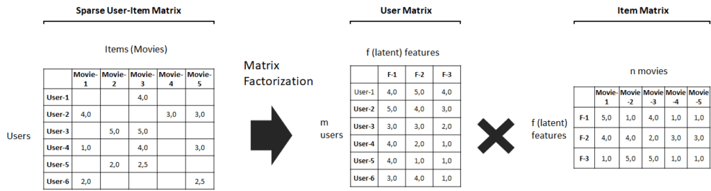
However, user/item matrices can become very large, making searching for patterns computationally expensive. Also, users will typically rate only a tiny fraction of the items in the matrix, so algorithms must deal with an abundant number of missing values (sparse matrix). Therefore, combining machine learning or deep learning with techniques for dimensionality reduction has become state-of-the-art.

One of the most widely used techniques for dimensionality reduction is matrix factorization. This approach compresses the initial sparse user/item matrix and presents it as separate matrices that present items and users as unknown feature vectors (as shown below). Such a matrix is densely populated and thus easier to handle, but it also enables the model to uncover latent dependencies among items and users, which increases model accuracy.

Python Libraries for Collaborative Filtering

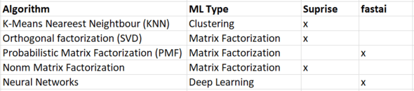
So far, only a few Python libraries support model-based collaborative Filtering out of the box. The most well-known libraries for recommender systems are probably Scikit-Suprise and Fast.ai for Pytorch.

Below you find an overview of the different algorithms that these libraries support.

Implementing a Movie Recommender in Python using Collaborative Filtering

Now it’s time to get our hands dirty and begin with implementing our movie recommender. As always, you find the code in the relataly git-hub repository.

Prerequisites

Before beginning the coding part, make sure that you have set up your Python 3 environment and required packages. If you don’t have an environment, consider the Anaconda Python environment. Follow this tutorial to set it up.

Also, make sure you install all required packages. In this tutorial, we will be working with the following standard packages: 

• pandas
• NumPy
• matplotlib

In addition, we will be using Seaborn for visualization and the recommender systems library Scikit-Suprise. You can install the surprise package by forging it with the following command:

• conda install -c conda-forge scikit-surprise

You can install the other packages using standard console commands:

• pip install <package name>
• conda install <package name> (if you are using the anaconda packet manager)

About the IMDB Movies Dataset

We will train our movie recommendation model on a popular Movies Dataset (you can download it from grouplens.org). The MovieLens recommendation service collected the Dataset from 610 users between 1996 and 2018. Unpack the data into the working folder of your project.

The full Dataset contains metadata on over 45,000 movies and 26 million ratings from over 270,000 users. However, we will be working with a subset of the data “ratings_small.csv,” which contains 100,836 ratings from 700 users on 9742 movies.

The Dataset contains the following files, from which we will only use the first two (Source of the data description: Kaggle.com):

• movies_metadata.csv: The main Movies Metadata file contains information on 45,000 movies featured in the Full MovieLens Dataset. Features include posters, backdrops, budget, revenue, release dates, languages, production countries, and companies.
• ratings_small.csv: The subset of 100,000 ratings from 700 users on 9,000 movies. Each line corresponds to a single 5-star movie rating with half-star increments (0.5 – 5.0 stars).

There are several other files included that we won’t use.

Step #1: Load the Data

Ensure you have downloaded and unpacked the data and the required packages.

You can then load the movie data into our Python project using the code snippet below. We do not need all of the files in the movie dataset and only work with the following two.

• movies_metadata.csv
• ratings_small.csv

1.1 Load the Movies Data

First, we will load the movies_metadata, which contains a list of all movies and meta information such as the release year, a short description, etc.

import numpy as np
import pandas as pd
import matplotlib.pyplot as plt
import seaborn as sns
from datetime import datetime
from surprise import SVD, Dataset, Reader
from surprise.model_selection import train_test_split, cross_validate
from ast import literal_eval

# in case you have placed the files outside of your working directory, you need to specify a path
path = '' # for example: 'data/movie_recommendations/'  

# load the movie metadata
df_moviesmetadata=pd.read_csv(path + 'movies_metadata.csv', low_memory=False) 
print(df_moviesmetadata.shape)
print(df_moviesmetadata.columns)
df_moviesmetadata.head(1)

(45466, 24)
Index(['adult', 'belongs_to_collection', 'budget', 'genres', 'homepage', 'id',
       'imdb_id', 'original_language', 'original_title', 'overview',
       'popularity', 'poster_path', 'production_companies',
       'production_countries', 'release_date', 'revenue', 'runtime',
       'spoken_languages', 'status', 'tagline', 'title', 'video',
       'vote_average', 'vote_count'],
      dtype='object')
	adult	belongs_to_collection								budget		genres												homepage								id	imdb_id		original_language	original_title	overview	...	release_date	revenue	runtime	spoken_languages	status	tagline	title	video	vote_average	vote_count
0	False	{'id': 10194, 'name': 'Toy Story Collection', ...	30000000	[{'id': 16, 'name': 'Animation'}, {'id': 35, '...	http://toystory.disney.com/toy-story	862	tt0114709	en					Toy Story		Led by Woody, Andy's toys live happily in his ...	...	1995-10-30	373554033.0	81.0	[{'iso_639_1': 'en', 'name': 'English'}]	Released	NaN	Toy Story	False	7.7	5415.0
1 rows × 24 columns

1.2 Load the Ratings Data

We proceed by loading the rating file. This file contains the movie ratings for each user, the movieId, and a timestamp.

In addition, we print the value counts for rankings in our Dataset.

# load the movie ratings
df_ratings=pd.read_csv(path + 'ratings_small.csv', low_memory=False) 

print(df_ratings.shape)
print(df_ratings.columns)
df_ratings.head(3)

rankings_count = df_ratings.rating.value_counts().sort_values()
sns.barplot(x=rankings_count.index.sort_values(), y=rankings_count, color="b")
sns.set_theme(style="whitegrid")

(100004, 4)
Index(['userId', 'movieId', 'rating', 'timestamp'], dtype='object')
	userId	movieId	rating	timestamp
0	1		31		2.5		1260759144
1	1		1029	3.0		1260759179
2	1		1061	3.0		1260759182

As we can see, most of the ratings in our Dataset are positive.

Step #2 Preprocessing and Cleaning the Data

We continue with the preprocessing of the data. The recommendations of a User-based Collaborative Filtering Approach rely solely on the interactions between users and items. This means training a prediction model does not require the meta-information of the movies. Nevertheless, we will load the metadata because it is just nicer to display the recommendations, movie title, release year, and so on, instead of just ids.

2.1 Clean the Movie Data

Unfortunately, the data quality of the movies’ metadata is not excellent, so we need to fix a few things. The following operations will change some data types to integers, extract the release year and genres, and remove some records with incorrect data.

# remove invalid records with invalid ids
df_mmeta = df_moviesmetadata.drop([19730, 29503, 35587])

df_movies = pd.DataFrame()

# extract the release year 
df_movies['year'] = pd.to_datetime(df_mmeta['release_date'], errors='coerce').apply(lambda x: str(x).split('-')[0] if x != np.nan else np.nan)

# extract genres
df_movies['genres'] = df_mmeta['genres'].fillna('[]').apply(literal_eval).apply(lambda x: [i['name'] for i in x] if isinstance(x, list) else [])

# change the index to movie_id
df_movies['movieId'] = pd.to_numeric(df_mmeta['id'])
df_movies = df_movies.set_index('movieId')

# add vote count
df_movies['vote_count'] = df_movies['vote_count'].astype('int')
df_movies

title									vote_count	vote_average	year	genres
		movieId					
862		Toy Story						5415			7.7	1995	[Animation, Comedy, Family]
8844	Jumanji							2413			6.9	1995	[Adventure, Fantasy, Family]
15602	Grumpier Old Men				92				6.5	1995	[Romance, Comedy]
31357	Waiting to Exhale				34				6.1	1995	[Comedy, Drama, Romance]
11862	Father of the Bride Part II		173				5.7	1995	[Comedy]
...	...	...	...	...	...
49279	The Man with the Rubber Head	29				7.6	1901	[Comedy, Fantasy, Science Fiction]
49271	The Devilish Tenant				12				6.7	1909	[Fantasy, Comedy]
49280	The One-Man Band				22				6.5	1900	[Fantasy, Action, Thriller]
404604	Mom								14				6.6	2017	[Crime, Drama, Thriller]
30840	Robin Hood						26				5.7	1991	[Drama, Action, Romance]
22931 rows × 5 columns

2.2 Clean the Ratings Data

Compared to the movie metadata, not much more needs to be done to the rating data. Here we just put the timestamp into a readable format.

One of the following steps is to use the Reader class from the Surprise library to parse the ratings and put them into a format compatible with standard recommendation algorithms from the Surprise library. The Reader needs the data in the form where each line contains only one rating and respects the following structure:

user; item ; rating ; timestamp

# drop na values
df_ratings_temp = df_ratings.dropna()

# convert datetime
df_ratings_temp['timestamp'] = pd. to_datetime(df_ratings_temp['timestamp'], unit='s')

print(f'unique users: {len(df_ratings_temp.userId.unique())}, ratings: {len(df_ratings_temp)}')
df_ratings_temp.head()

unique users: 671, ratings: 100004
	userId		movieId	rating	timestamp
0	1			31		2.5		2009-12-14 02:52:24
1	1			1029	3.0		2009-12-14 02:52:59
2	1			1061	3.0		2009-12-14 02:53:02
3	1			1129	2.0		2009-12-14 02:53:05
4	1			1172	4.0		2009-12-14 02:53:25

Step #3: Split the Data in Train and Test

Next, we will split the data into train and test sets. In this way, we ensure that we can later evaluate the performance of our recommender model on data that the model has not yet seen.

# The Reader class is used to parse a file containing ratings.
# The file is assumed to specify only one rating per line, such as in the df_ratings_temp file above.
reader = Reader()
ratings_by_users = Dataset.load_from_df(df_ratings_temp[['userId', 'movieId', 'rating']], reader)

# Split the Data into train and test
train_df, test_df = train_test_split(ratings_by_users, test_size=.2)

Once we have split the data into train and test, we can train the recommender model.

Step #4: Train a Movie Recommender using Collaborative Filtering

Training the SVD model requires only lines of code. The first line creates an untrained model that uses Probabilistic Matrix Factorization for dimensionality reduction. The second line will fit this model to the training data.

# train an SVD model
svd_model = SVD()
svd_model_trained = svd_model.fit(train_df)

Step #5: Evaluate Prediction Performance using Cross-Validation

Next, it is time to validate the performance of our movie recommendation program. For this, we use k-fold cross-validation. As a reminder, cross-validation involves splitting the Dataset into different folds and then measuring the prediction performance based on each fold.

We can measure model performance using indicators such as mean absolute error (MAE) or mean squared error (MSE). The MAE is the average difference between predicting a movie and the actual ratings. We chose this measure because it is easy to understand.

# 10-fold cross validation 
cross_val_results = cross_validate(svd_model_trained, ratings_by_users, measures=['RMSE', 'MAE', 'MSE'], cv=10, verbose=False)
test_mae = cross_val_results['test_mae']

# mean squared errors per fold
df_test_mae = pd.DataFrame(test_mae, columns=['Mean Absolute Error'])
df_test_mae.index = np.arange(1, len(df_test_mae) + 1)
df_test_mae.sort_values(by='Mean Absolute Error', ascending=False).head(15)

# plot an overview of the performance per fold
plt.figure(figsize=(6,4))
sns.set_theme(style="whitegrid")
sns.barplot(y='Mean Absolute Error', x=df_test_mae.index, data=df_test_mae, color="b")
# plt.title('Mean Absolute Error')

The chart above shows that the mean deviation of our predictions from the actual rating is a little below 0.7. The result is not terrific but ok for a first model. In addition, there are no significant differences between the performance in the different folds. Let’s keep in mind that the MAE says little about possible outliers in the predictions. However, since we are dealing with ordinal predictions (1-5), the influence of outliers is naturally limited.

Step #6: Generate Predictions

Finally, we will use our movie recommender to generate a list of suggested movies for a specific test user. The predictions will be based on the user’s previous movie ratings.

# predict ratings for a single user_id and for all movies
user_id = 400 # some test user from the ratings file

# create the predictions
pred_series= []
df_ratings_filtered = df_ratings[df_ratings['userId'] == user_id]

print(f'number of ratings: {df_ratings_filtered.shape[0]}')
for movie_id, name in zip(df_movies.index, df_movies['title']):
    # check if the user has already rated a specific movie from the list
    rating_real = df_ratings.query(f'movieId == {movie_id}')['rating'].values[0] if movie_id in df_ratings_filtered['movieId'].values else 0
    # generate the prediction
    rating_pred = svd_model_trained.predict(user_id, movie_id, rating_real, verbose=False)
    # add the prediction to the list of predictions
    pred_series.append([movie_id, name, rating_pred.est, rating_real])

# print the results
df_recommendations = pd.DataFrame(pred_series, columns=['movieId', 'title', 'predicted_rating', 'actual_rating'])
df_recommendations.sort_values(by='predicted_rating', ascending=False).head(15)

		movieId	title								predicted_rating	actual_rating
4234	4993	5 Card Stud							4.721481			0.0
3194	318		The Million Dollar Hotel			4.648623			5.0
442		858		Sleepless in Seattle				4.506962			0.0
236		527		Once Were Warriors					4.484758			4.0
2426	926		Galaxy Quest						4.465653			0.0
6532	905		Pandora's Box						4.452688			0.0
710		260		The 39 Steps						4.390318			0.0
8787	3683	Flags of Our Fathers				4.386821			0.0
5400	899		Broken Blossoms						4.384220			0.0
5068	296		Terminator 3: Rise of the Machines	4.383057			4.0
372		2019	Hard Target							4.365834			0.0
7254	919		Blood: The Last Vampire				4.356012			0.0
3295	4973	Under the Sand						4.355750			0.0
3869	194		Amélie								4.353614			0.0
8631	1948	Crank								4.344286			0.0

Alternatively, we can predict how well a specific user will rate a movie by handing the user_id and the movie_id to the model.

# predict ratings for the combination of user_id and movie_id
user_id = 217 # some test user from the ratings file
movie_id = 4002
rating_real = df_ratings.query(f'movieId == {movie_id} & userId == {user_id}')['rating'].values[0]
movie_title = df_movies[df_movies.index == 862]['title'].values[0]

print(f'Movie title: {movie_title}')
print(f'Actual rating: {rating_real}')

# predict and show the result
rating_pred = svd_model_trained.predict(user_id, movie_id, rating_real, verbose=True)

Movie title: Toy Story
Actual rating: 4.5
user: 217        item: 4002       r_ui = 4.50   est = 3.98   {'was_impossible': False}

Summary

Congratulations on learning how to develop a movie recommendation system in Python! In this article, you learned about the SVD model, which uses matrix factorization and collaborative filtering to predict movie ratings for a given user. We also demonstrated how to perform cross-validation on a movie dataset and use the model to generate movie recommendations.

Several other approaches can be used to develop a movie recommendation system, including content-based filtering, which uses features of the movies themselves (such as genre, director, and cast) to make recommendations, and hybrid systems, which combine the strengths of multiple approaches.

Regardless of the approach used, building a movie recommendation system can be a useful tool for recommending movies to users based on their past preferences and can help increase engagement and satisfaction with a movie streaming service or website.

If you like the post, please let me know in the comments, and don’t forget to subscribe to our Twitter account to stay up to date on upcoming articles.

Sources and Further Reading

Below are some resources for further reading on recommender systems and content-based models.

Books

1. Charu C. Aggarwal (2016) Recommender Systems: The Textbook
2. Kin Falk (2019) Practical Recommender Systems
3. Andriy Burkov (2020) Machine Learning Engineering
4. Oliver Theobald (2020) Machine Learning For Absolute Beginners: A Plain English Introduction
5. Aurélien Géron (2019) Hands-On Machine Learning with Scikit-Learn, Keras, and TensorFlow: Concepts, Tools, and Techniques to Build Intelligent Systems
6. David Forsyth (2019) Applied Machine Learning Springer

The links above to Amazon are affiliate links. By buying through these links, you support the Relataly.com blog and help to cover the hosting costs. Using the links does not affect the price.

Articles

1. Getting started with Suprise
2. About the history of Recommender Systems
3. Singular value decomposition vs. matrix factorization
4. Probabilistic Matrix Factorization