Multivariate Anomaly Detection on Time-Series Data in Python: Using Isolation Forests to Detect Credit Card Fraud

Credit card fraud has become one of the most common use cases for anomaly detection systems. The number of fraud attempts has risen sharply, resulting in billions of dollars in losses. Early detection of fraud attempts with machine learning is therefore becoming increasingly important. In this article, we take on the fight against international credit card fraud and develop a multivariate anomaly detection model in Python that spots fraudulent payment transactions. The model will use the Isolation Forest algorithm, one of the most effective techniques for detecting outliers. Isolation Forests are so-called ensemble models. They have various hyperparameters with which we can optimize model performance. However, we will not do this manually but instead, use grid search for hyperparameter tuning. To assess the performance of our model, we will also compare it with other models.

The remainder of this article is structured as follows: We start with a brief introduction to anomaly detection and look at the Isolation Forest algorithm. Equipped with these theoretical foundations, we then turn to the practical part, in which we train and validate an isolation forest that detects credit card fraud. We use an unsupervised learning approach, where the model learns to distinguish regular from suspicious card transactions. We will train our model on a public dataset from Kaggle that contains credit card transactions. Finally, we will compare the performance of our model against two nearest neighbor algorithms (LOF and KNN).

Multivariate Anomaly Detection

Before we take a closer look at the use case and our unsupervised approach, let’s briefly discuss anomaly detection. Anomaly detection deals with finding points that deviate from legitimate data regarding their mean or median in a distribution. In machine learning, the term is often used synonymously with outlier detection.

Some anomaly detection models work with a single feature (univariate data), for example, in monitoring electronic signals. However, most anomaly detection models use multivariate data, which means they have two (bivariate) or more (multivariate) features. They find a wide range of applications, including the following:

• Predictive Maintenance and Detection of Malfunctions and Decay
• Detection of Retail Bank Credit Card Fraud
• Detection of Pricing Errors
• Cyber Security, for example, Network Intrusion Detection
• Detecting Fraudulent Market Behavior in Investment Banking

Unsupervised Algorithms for Anomaly Detection

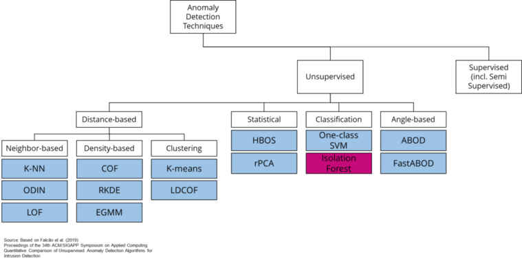
Outlier detection is a classification problem. However, the field is more diverse as outlier detection is a problem we can approach with supervised and unsupervised machine learning techniques. It would go beyond the scope of this article to explain the multitude of outlier detection techniques. Still, the following chart provides a good overview of standard algorithms that learn unsupervised.

A prerequisite for supervised learning is that we have information about which data points are outliers and belong to regular data. In credit card fraud detection, this information is available because banks can validate with their customers whether a suspicious transaction is a fraud or not. In many other outlier detection cases, it remains unclear which outliers are legitimate and which are just noise or other uninteresting events in the data.

Whether we know which classes in our dataset are outliers and which are not affects the selection of possible algorithms we could use to solve the outlier detection problem. Unsupervised learning techniques are a natural choice if the class labels are unavailable. And if the class labels are available, we could use both unsupervised and supervised learning algorithms.

In the following, we will focus on Isolation Forests.

The Isolation Forest (“iForest”) Algorithm

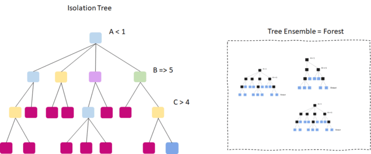
Isolation forests (sometimes called iForests) are among the most powerful techniques for identifying anomalies in a dataset. They belong to the group of so-called ensemble models. The predictions of ensemble models do not rely on a single model. Instead, they combine the results of multiple independent models (decision trees). Nevertheless, isolation forests should not be confused with traditional random decision forests. While random forests predict given class labels (supervised learning), isolation forests learn to distinguish outliers from inliers (regular data) in an unsupervised learning process.

An Isolation Forest contains multiple independent isolation trees. The algorithm invokes a process that recursively divides the training data at random points to isolate data points from each other to build an Isolation Tree. The number of partitions required to isolate a point tells us whether it is an anomalous or regular point. The underlying assumption is that random splits can isolate an anomalous data point much sooner than nominal ones.

Also: Stock Market Prediction using Multivariate Time Series Data

How the Isolation Forest Algorithm Works

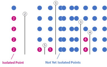
The illustration below shows exemplary training of an Isolation Tree on univariate data, i.e., with only one feature. The algorithm has already split the data at five random points between the minimum and maximum values of a random sample. The isolated points are colored in purple. The example below has taken two partitions to isolate the point on the far left. The other purple points were separated after 4 and 5 splits.

The partitioning process ends when the algorithm has isolated all points from each other or when all remaining points have equal values. The algorithm has calculated and assigned an outlier score to each point at the end of the process, based on how many splits it took to isolate it.

When using an isolation forest model on unseen data to detect outliers, the algorithm will assign an anomaly score to the new data points. These scores will be calculated based on the ensemble trees we built during model training.

So how does this process work when our dataset involves multiple features? For multivariate anomaly detection, partitioning the data remains almost the same. The significant difference is that the algorithm selects a random feature in which the partitioning will occur before each partitioning. Consequently, multivariate isolation forests split the data along multiple dimensions (features).

Credit Card Fraud Detection using Isolation Forests

Monitoring transactions has become a crucial task for financial institutions. In 2019 alone, more than 271,000 cases of credit card theft were reported in the U.S., causing billions of dollars in losses and making credit card fraud one of the most common types of identity theft. The vast majority of fraud cases are attributable to organized crime, which often specializes in this particular crime.

Anything that deviates from the customer’s normal payment behavior can make a transaction suspicious, including an unusual location, time, or country in which the customer conducted the transaction. Credit card providers use similar anomaly detection systems to monitor their customers’ transactions and look for potential fraud attempts. They can halt the transaction and inform their customer as soon as they detect a fraud attempt. We train an Isolation Forest algorithm for credit card fraud detection using Python in the following.

Now that we have established the context for our machine learning problem, we can begin implementing an anomaly detection model in Python.

The code is available on the GitHub repository.

View on GitHub Relataly GitHub Repo

Prerequisites

Before starting the coding part, make sure that you have set up your Python 3 environment and required packages. If you don’t have an environment, consider the Anaconda Python environment. To set it up, you can follow the steps in this tutorial.

Also, make sure you install all required packages. In this tutorial, we will be working with the following standard packages: 

• pandas
• NumPy
• matplotlib

In addition, we will be using the machine learning library Scikit-learn and Seaborn for visualization.

You can install packages using console commands:

• pip install <package name>
• conda install <package name> (if you are using the anaconda packet manager)

Dataset: Credit Card Transactions

In the following, we will work with a public dataset containing anonymized credit card transactions made by European cardholders in September 2013. You can download the dataset from Kaggle.com.

The dataset contains 28 features (V1-V28) obtained from the source data using Principal Component Analysis (PCA). In addition, the data includes the date and the amount of the transaction.

Transactions are labeled fraudulent or genuine, with 492 fraudulent cases out of 284,807 transactions. The positive class (frauds) accounts for only 0.172% of all credit card transactions, so the classes are highly unbalanced.

Step #1: Load the Data

In the following, we will go through several steps of training an Anomaly detection model for credit card fraud. We will carry out several activities, such as:

1. Loading and preprocessing the data: this involves cleaning, transforming, and preparing the data for analysis, in order to make it suitable for use with the isolation forest algorithm.
2. Feature engineering: this involves extracting and selecting relevant features from the data, such as transaction amounts, merchant categories, and time of day, in order to create a set of inputs for the anomaly detection algorithm.
3. Model training: We will train several machine learning models on different algorithms (incl. the isolation forest) on the preprocessed and engineered data. The models will learn the normal patterns and behaviors in credit card transactions. This activity includes hyperparameter tuning.
4. Model evaluation and testing: this involves evaluating the performance of the trained model on a test dataset in order to assess its accuracy, precision, recall, and other metrics and to identify any potential issues or improvements. As part of this activity, we compare the performance of the isolation forest to other models.

We begin by setting up imports and loading the data into our Python project. Then we’ll quickly verify that the dataset looks as expected.

import math 
import numpy as np 
import pandas as pd 
import matplotlib.pyplot as plt
from datetime import date, timedelta, datetime
import seaborn as sns
from sklearn.ensemble import IsolationForest
from sklearn.model_selection import train_test_split
from sklearn.neighbors import LocalOutlierFactor, KNeighborsClassifier
from sklearn.metrics import accuracy_score, confusion_matrix, classification_report, plot_confusion_matrix

# The Data can be downloaded from Kaggle.com: https://www.kaggle.com/mlg-ulb/creditcardfraud?select=creditcard.csv
path = 'data/credit-card-transactions/'
df = pd.read_csv(f'{path}creditcard.csv')
df

		Time	V1			V2			V3			V4			V5			V6			V7			V8			V9			...	V21	V22	V23	V24	V25	V26	V27	V28	Amount	Class
0		0.0		-1.359807	-0.072781	2.536347	1.378155	-0.338321	0.462388	0.239599	0.098698	0.363787	...	-0.018307	0.277838	-0.110474	0.066928	0.128539	-0.189115	0.133558	-0.021053	149.62	0
1		0.0		1.191857	0.266151	0.166480	0.448154	0.060018	-0.082361	-0.078803	0.085102	-0.255425	...	-0.225775	-0.638672	0.101288	-0.339846	0.167170	0.125895	-0.008983	0.014724	2.69	0
2		1.0		-1.358354	-1.340163	1.773209	0.379780	-0.503198	1.800499	0.791461	0.247676	-1.514654	...	0.247998	0.771679	0.909412	-0.689281	-0.327642	-0.139097	-0.055353	-0.059752	378.66	0
3		1.0		-0.966272	-0.185226	1.792993	-0.863291	-0.010309	1.247203	0.237609	0.377436	-1.387024	...	-0.108300	0.005274	-0.190321	-1.175575	0.647376	-0.221929	0.062723	0.061458	123.50	0
4		2.0		-1.158233	0.877737	1.548718	0.403034	-0.407193	0.095921	0.592941	-0.270533	0.817739	...	-0.009431	0.798278	-0.137458	0.141267	-0.206010	0.502292	0.219422	0.215153	69.99	0
...	...	...	...	...	...	...	...	...	...	...	...	...	...	...	...	...	...	...	...	...	...
284802	172786.0	-11.881118	10.071785	-9.834783	-2.066656	-5.364473	-2.606837	-4.918215	7.305334	1.914428	...	0.213454	0.111864	1.014480	-0.509348	1.436807	0.250034	0.943651	0.823731	0.77	0
284803	172787.0	-0.732789	-0.055080	2.035030	-0.738589	0.868229	1.058415	0.024330	0.294869	0.584800	...	0.214205	0.924384	0.012463	-1.016226	-0.606624	-0.395255	0.068472	-0.053527	24.79	0
284804	172788.0	1.919565	-0.301254	-3.249640	-0.557828	2.630515	3.031260	-0.296827	0.708417	0.432454	...	0.232045	0.578229	-0.037501	0.640134	0.265745	-0.087371	0.004455	-0.026561	67.88	0
284805	172788.0	-0.240440	0.530483	0.702510	0.689799	-0.377961	0.623708	-0.686180	0.679145	0.392087	...	0.265245	0.800049	-0.163298	0.123205	-0.569159	0.546668	0.108821	0.104533	10.00	0
284806	172792.0	-0.533413	-0.189733	0.703337	-0.506271	-0.012546	-0.649617	1.577006	-0.414650	0.486180	...	0.261057	0.643078	0.376777	0.008797	-0.473649	-0.818267	-0.002415	0.013649	217.00	0

Everything should look good so that we can continue.

Step #2: Data Exploration

The purpose of data exploration in anomaly detection is to gain a better understanding of the data and the underlying patterns and trends that it contains. This can help to identify potential anomalies or outliers in the data and to determine the appropriate approaches and algorithms for detecting them.

In the following, we will create histograms that visualize the distribution of the different features.

2.1 Features

First, we will create a series of frequency histograms for our dataset’s features (V1 – V28). We will subsequently take a different look at the Class, Time, and Amount so that we can drop them at the moment.

# create histograms on all features
df_hist = df_base.drop(['Time','Amount', 'Class'], 1)
df_hist.hist(figsize=(20,20), bins = 50, color = "c", edgecolor='black')
plt.show()

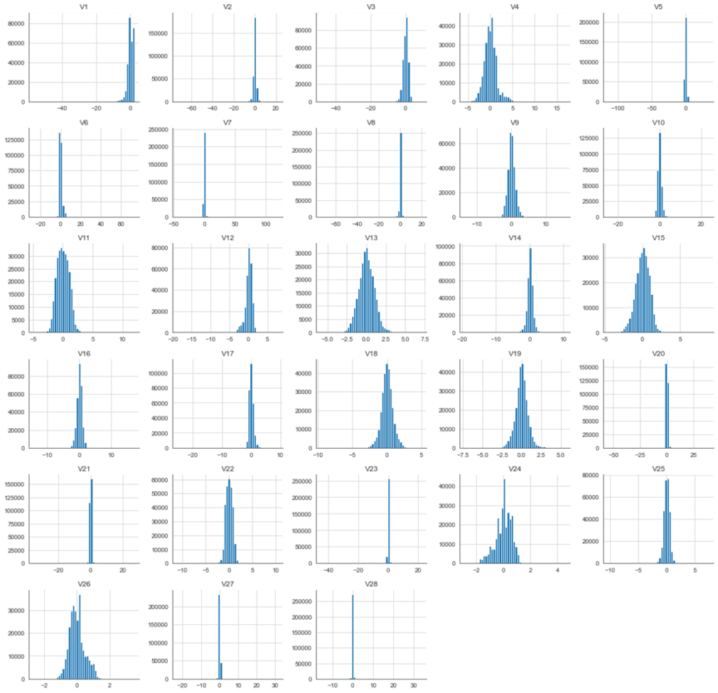
Next, we will look at the correlation between the 28 features. We expect the features to be uncorrelated due to the use of PCA. Let’s verify that by creating a heatmap on their correlation values.

# feature correlation
f_cor = df_hist.corr()
sns.heatmap(f_cor)

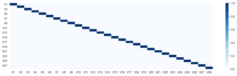
As we expected, our features are uncorrelated.

2.2 Class Labels

Next, let’s print an overview of the class labels to understand better how balanced the two classes are.

# Plot the balance of class labels
fig1, ax1 = plt.subplots(figsize=(14, 7))
plt.pie(df[['Class']].value_counts(), explode=[0,0.1], labels=[0,1], autopct='%1.2f%%', shadow=True, startangle=45)

We see that the data set is highly unbalanced. While this would constitute a problem for traditional classification techniques, it is a predestined use case for outlier detection algorithms like the Isolation Forest.

2.3 Time and Amount

Finally, we will create some plots to gain insights into time and amount. Let’s first have a look at the time variable.

# Plot istribution of the Time variable, which contains transaction data for two days
fig, ax = plt.subplots(nrows=1, ncols=2, sharex=True, figsize=(14, 7))
sns.histplot(data=df_base[df_base['Class'] == 0], x='Time', kde=True, ax=ax[0])
sns.histplot(data=df_base[df_base['Class'] == 1], x='Time', kde=True, ax=ax[1])
plt.show()

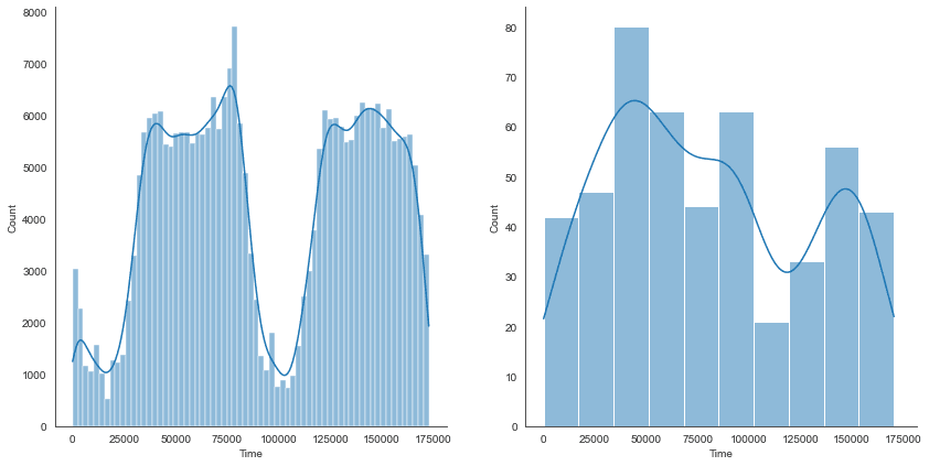
The time frame of our dataset covers two days, which reflects the distribution graph well. We can see that most transactions happen during the day – which is only plausible.

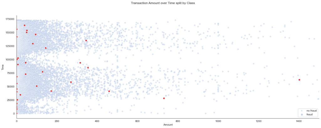
Next, let’s examine the correlation between transaction size and fraud cases. To do this, we create a scatterplot that distinguishes between the two classes.

# Plot time against amount
x = df_base['Amount']
y = df_base['Time']
fig, ax = plt.subplots(figsize=(20, 7))
ax.set(xlim=(0, 1500))
sns.scatterplot(data=df_base[df_base['Class']==0][::15], x=x, y=y, hue="Class", palette=["#BECEE9"], alpha=.5, ax=ax)
sns.scatterplot(data=df_base[df_base['Class']==1][::15], x=x, y=y, hue="Class", palette=["#EF1B1B"], zorder=100, ax=ax)
plt.legend(['no fraud', 'fraud'], loc='lower right')
fig.suptitle('Transaction Amount over Time split by Class')

The scatterplot provides the insight that suspicious amounts tend to be relatively low. In other words, there is some inverse correlation between class and transaction amount.

Step #3: Preprocessing

Now that we have a rough idea of the data, we will prepare it for training the model. For the training of the isolation forest, we drop the class label from the base dataset and then divide the data into separate datasets for training (70%) and testing (30%). We do not have to normalize or standardize the data when using a decision tree-based algorithm.

We will use all features from the dataset. So our model will be a multivariate anomaly detection model.

# Separate the classes from the train set
df_classes = df_base['Class']
df_train = df_base.drop(['Class'], axis=1)

# split the data into train and test 
X_train, X_test, y_train, y_test = train_test_split(df_train, df_classes, test_size=0.30, random_state=42)

Step #4: Model Training

Once we have prepared the data, it’s time to start training the Isolation Forest. However, to compare the performance of our model with other algorithms, we will train several different models. In total, we will prepare and compare the following five outlier detection models:

• Isolation Forest (default)
• Isolation Forest (hypertuned)
• Local Outlier Factor (default)
• K Neared Neighbour (default)
• K Nearest Neighbour (hypertuned)

For hyperparameter tuning of the models, we use Grid Search.

4.1 Train an Isolation Forest

Next, we train our isolation forest algorithm. An isolation forest is a type of machine learning algorithm for anomaly detection. It is a variant of the random forest algorithm, which is a widely-used ensemble learning method that uses multiple decision trees to make predictions.

The isolation forest algorithm works by randomly selecting a feature and a split value for the feature, and then using the split value to divide the data into two subsets. This process is repeated for each decision tree in the ensemble, and the trees are combined to make a final prediction.

The isolation forest algorithm is designed to be efficient and effective for detecting anomalies in high-dimensional datasets. It has a number of advantages, such as its ability to handle large and complex datasets, and its high accuracy and low false positive rate. It is widely used in a variety of applications, such as fraud detection, intrusion detection, and anomaly detection in manufacturing.

4.1.1 Isolation Forest (baseline)

First, we train a baseline model. A baseline model is a simple or reference model used as a starting point for evaluating the performance of more complex or sophisticated models in machine learning. It provides a baseline or benchmark for comparison, which allows us to assess the relative performance of different models and to identify which models are more accurate, effective, or efficient.

# train the model on the nominal train set
model_isf = IsolationForest().fit(X_train)

We create a function to measure the performance of our baseline model and illustrate the results in a confusion matrix. Later, when we go into hyperparameter tuning, we can use this function to objectively compare the performance of more sophisticated models.

def measure_performance(model, X_test, y_true, map_labels):
    # predict on testset
    df_pred_test = X_test.copy()
    #df_pred_test['Class'] = y_test
    df_pred_test['Pred'] = model.predict(X_test)
    if map_labels:
        df_pred_test['Pred'] = df_pred_test['Pred'].map({1: 0, -1: 1})
    #df_pred_test['Outlier_Score'] = model.decision_function(X_test)

    # measure performance
    #y_true = df_pred_test['Class']
    x_pred = df_pred_test['Pred'] 
    matrix = confusion_matrix(x_pred, y_true)

    sns.heatmap(pd.DataFrame(matrix, columns = ['Actual', 'Predicted']),
                xticklabels=['Regular [0]', 'Fraud [1]'], 
                yticklabels=['Regular [0]', 'Fraud [1]'], 
                annot=True, fmt="d", linewidths=.5, cmap="YlGnBu")
    plt.ylabel('Predicted')
    plt.xlabel('Actual')
    
    print(classification_report(x_pred, y_true))
    
    model_score = score(x_pred, y_true,average='macro')
    print(f'f1_score: {np.round(model_score[2]*100, 2)}%')
    
    return model_score

model_name = 'Isolation Forest (baseline)'
print(f'{model_name} model')

map_labels = True
model_score = measure_performance(model_isf, X_test, y_test, map_labels)

performance_df = pd.DataFrame().append({'model_name':model_name, 
                                    'f1_score': model_score[0], 
                                    'precision': model_score[1], 
                                    'recall': model_score[2]}, ignore_index=True)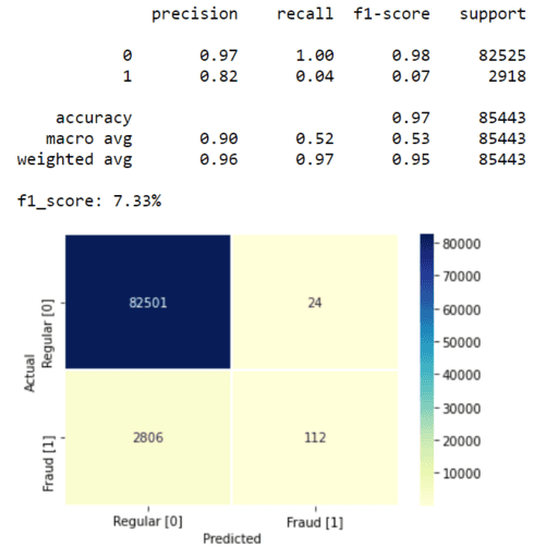

4.1.2 Isolation Forest (Hypertuning)

Next, we will train another Isolation Forest Model using grid search hyperparameter tuning to test different parameter configurations.

The hyperparameters of an isolation forest include:

• n_estimators: The number of decision trees in the forest.
• max_samples: The number of samples to draw from the dataset to train each decision tree.
• contamination: The expected proportion of anomalies in the dataset.
• max_features: The number of features to consider when choosing the split points in the decision trees.
• bootstrap: Whether or not to use bootstrap sampling when drawing samples to train the decision trees.

These hyperparameters can be adjusted to improve the performance of the isolation forest. The optimal values for these hyperparameters will depend on the specific characteristics of the dataset and the task at hand, which is why we require several experiments.

The code below will evaluate the different parameter configurations based on their f1_score and automatically choose the best-performing model.

# Define the parameter grid
n_estimators=[50, 100]
max_features=[1.0, 5, 10]
bootstrap=[True]
param_grid = dict(n_estimators=n_estimators, max_features=max_features, bootstrap=bootstrap)

# Build the gridsearch
model_isf = IsolationForest(n_estimators=n_estimators, 
                            max_features=max_features, 
                            contamination=contamination_rate, 
                            bootstrap=False, 
                            n_jobs=-1)

# Define an f1_scorer
f1sc = make_scorer(f1_score, average='macro')

grid = GridSearchCV(estimator=model_isf, param_grid=param_grid, cv = 3, scoring=f1sc)
grid_results = grid.fit(X=X_train, y=y_train)

# Summarize the results in a readable format
print("Best: {0}, using {1}".format(grid_results.cv_results_['mean_test_score'], grid_results.best_params_))
results_df = pd.DataFrame(grid_results.cv_results_)

# Evaluate model performance
model_name = 'KNN (tuned)'
print(f'{model_name} model')

best_model = grid_results.best_estimator_
map_labels = True # if True - maps 1 to 0 and -1 to 1 - not required for scikit-learn knn models
model_score = measure_performance(best_model, X_test, y_test, map_labels)
performance_df = performance_df.append({'model_name':model_name, 
                                    'f1_score': model_score[0], 
                                    'precision': model_score[1], 
                                    'recall': model_score[2]}, ignore_index=True)
results_df

Best: [0.61083219 0.55718259 0.55912644 0.52670328 0.5317127 ], using {'n_neighbors': 1}
KNN (tuned) model
              precision    recall  f1-score   support

           0       1.00      1.00      1.00     85385
           1       0.21      0.48      0.29        58

    accuracy                           1.00     85443
   macro avg       0.60      0.74      0.64     85443
weighted avg       1.00      1.00      1.00     85443

f1_score: 64.39%

4.2 LOF Model

We train the Local Outlier Factor Model using the same training data and evaluation procedure. The local outlier factor (LOF) is a measure of the local deviation of a data point with respect to its neighbors. It is used to identify points in a dataset that are significantly different from their surrounding points and that may therefore be considered outliers.

The LOF is a useful tool for detecting outliers in a dataset, as it considers the local context of each data point rather than the global distribution of the data. This makes it more robust to outliers that are only significant within a specific region of the dataset. However, isolation forests can often outperform LOF models.

# Train a tuned local outlier factor model
model_lof = LocalOutlierFactor(n_neighbors=3, contamination=contamination_rate, novelty=True)
model_lof.fit(X_train)

# Evaluate model performance
model_name = 'LOF (baseline)'
print(f'{model_name} model')

map_labels = True 
model_score = measure_performance(model_lof, X_test, y_test, map_labels)
performance_df = performance_df.append({'model_name':model_name, 
                                    'f1_score': model_score[0], 
                                    'precision': model_score[1], 
                                    'recall': model_score[2]}, ignore_index=True)

4.3 KNN Model

Next, we train the KNN models. KNN is a type of machine learning algorithm for classification and regression. It is a type of instance-based learning, which means that it stores and uses the training data instances themselves to make predictions, rather than building a model that summarizes or generalizes the data.

Below we add two K-Nearest Neighbor models to our list. We use the default parameter hyperparameter configuration for the first model. The second model will most likely perform better because we optimize its hyperparameters using the grid search technique.

4.3.1 KNN (default)

First, we train the default model using the same training data as before. By experimenting with different values of this parameter, you can try to identify the optimal number of neighbors that maximize the model’s performance on the given dataset. This approach could help to achieve better results compared to the default settings of the KNN algorithm, which may not be the most appropriate for the specific dataset we are working with.

# Train a KNN Model
model_knn = KNeighborsClassifier(n_neighbors=5)
model_knn.fit(X=X_train, y=y_train)

# Evaluate model performance
model_name = 'KNN (baseline)'
print(f'{model_name} model')

map_labels = False # if True - maps 1 to 0 and -1 to 1 - set to False for classification models (e.g., KNN)
model_score = measure_performance(model_knn, X_test, y_test, map_labels)
performance_df = performance_df.append({'model_name':model_name, 
                                    'f1_score': model_score[0], 
                                    'precision': model_score[1], 
                                    'recall': model_score[2]}, ignore_index=True)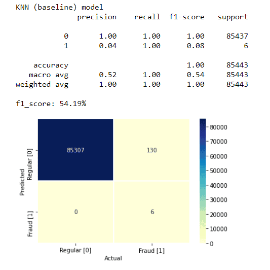

4.3.1 KNN (hypertuned)

In the next step, we will train a second KNN model to improve its performance by fine-tuning its hyperparameters. Despite having only a few parameters, hyperparameter tuning can enhance the model’s ability to make accurate predictions. In this case, we will concentrate on optimizing the number of nearest neighbors considered in the KNN algorithm.

# Define hypertuning parameters
n_neighbors=[1, 2, 3, 4, 5]
param_grid = dict(n_neighbors=n_neighbors)

# Build the gridsearch
model_knn = KNeighborsClassifier(n_neighbors=n_neighbors)
grid = GridSearchCV(estimator=model_knn, param_grid=param_grid, cv = 5)
grid_results = grid.fit(X=X_train, y=y_train)

# Summarize the results in a readable format
print("Best: {0}, using {1}".format(grid_results.cv_results_['mean_test_score'], grid_results.best_params_))
results_df = pd.DataFrame(grid_results.cv_results_)

# Evaluate model performance
model_name = 'KNN (tuned)'
print(f'{model_name} model')

best_model = grid_results.best_estimator_
map_labels = False # if True - maps 1 to 0 and -1 to 1 - set to False for classification models (e.g., KNN)
model_score = measure_performance(best_model, X_test, y_test, map_labels)
performance_df = performance_df.append({'model_name':model_name, 
                                    'f1_score': model_score[0], 
                                    'precision': model_score[1], 
                                    'recall': model_score[2]}, ignore_index=True)
results_df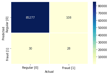

Step #5: Measuring and Comparing Performance

Finally, we will compare the performance of our models with a bar chart that shows the f1_score, precision, and recall. If you want to learn more about classification performance, this tutorial discusses the different metrics in more detail.

print(performance_df)

performance_df = performance_df.sort_values('model_name')

fig, ax = plt.subplots(figsize=(12, 4))
tidy = performance_df.melt(id_vars='model_name').rename(columns=str.title)
sns.barplot(y='Model_Name', x='Value', hue='Variable', data=tidy, ax=ax, palette='nipy_spectral', linewidth=1, edgecolor="w")
plt.title('Model Outlier Detection Performance (Macro)')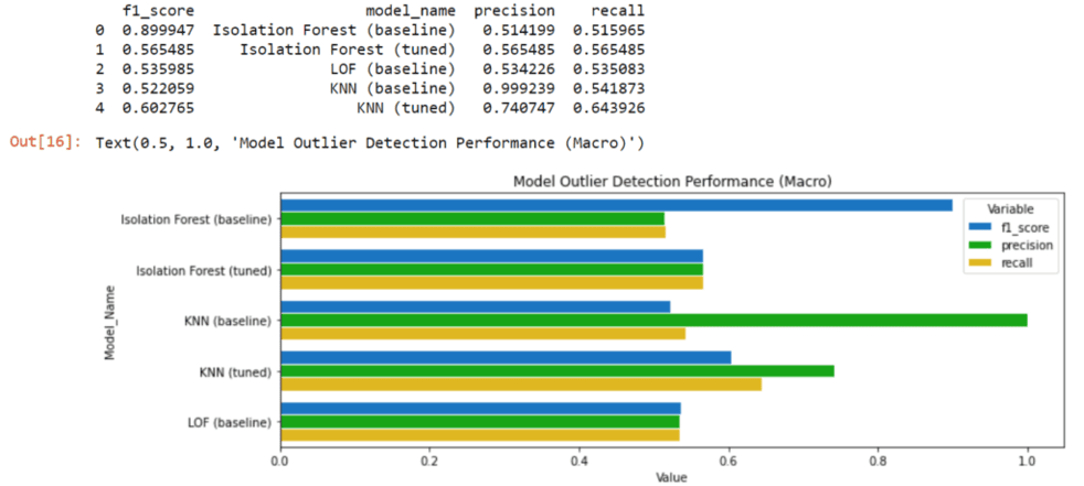

All three metrics play an important role in evaluating performance because, on the one hand, we want to capture as many fraud cases as possible, but we also don’t want to raise false alarms too frequently.

• As we can see, the optimized Isolation Forest performs particularly well-balanced.
• The default Isolation Forest has a high f1_score and detects many fraud cases but frequently raises false alarms.
• The opposite is true for the KNN model. Only a few fraud cases are detected here, but the model is often correct when noticing a fraud case.
• The default LOF model performs slightly worse than the other models. Compared to the optimized Isolation Forest, it performs worse in all three metrics.

Summary

Credit card fraud detection is important because it helps to protect consumers and businesses, to maintain trust and confidence in the financial system, and to reduce financial losses. It is a critical part of ensuring the security and reliability of credit card transactions.

This article has shown how to use Python and the Isolation Forest Algorithm to implement a credit card fraud detection system. We developed a multivariate anomaly detection model to spot fraudulent credit card transactions. You learned how to prepare the data for testing and training an isolation forest model and how to validate this model. Finally, we have proven that the Isolation Forest is a robust algorithm for anomaly detection that outperforms traditional techniques.

I hope you enjoyed the article and can apply what you learned to your projects. Have a great day!

Sources and Further Reading

The links above to Amazon are affiliate links. By buying through these links, you support the Relataly.com blog and help to cover the hosting costs. Using the links does not affect the price.