Image Classification with Convolutional Neural Networks – Classifying Cats and Dogs in Python

Image Classification with Convolutional Neural Networks

The history of image recognition dates back to the mid-1960s when the first attempts were made to identify objects by coding their characteristic shapes and lines. However, this task turned out to be incredibly complex. Our human brain is trained so well to recognize things that one can easily forget how diverse the observation conditions can be. Here are some examples:

• Fotos can be taken from various viewpoints
• Living things can have multiple forms and poses
• Objects come in different forms, colors, and sizes
• The picture may hide parts of the things in the picture
• The light conditions vary from image to image
• There may be one or multiple objects in the same image

At the beginning of the 1990s, the focus of research shifted to statistical approaches and learning algorithms.

The Emergence of CNNs

The basic concept of a neural network in computer vision has existed since the 1980s. It goes back to research from Hubel and Wiesel on the emergence of a cat’s visual system. They found that the visual cortex has cells activated by specific shapes and their orientation in the visual field. Some of their findings inspired the development of crucial computer vision technologies, such as, for example, hierarchical features with different levels of abstraction [1, 2]. However, it took another three decades of research and the availability of faster computers before the emergence of modern CNNs.

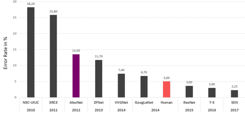
The year 2012 was a defining moment for the use of CNNs in image recognition. This year, for the first time, CNN won the ILSVRC competition for computer vision. The challenge was classifying more than a hundred thousand images into 1000 object categories. With an error rate of only 15,3%, the succeeding model was a CNN called “AlexNet.”.

AlexNet was the first model to achieve more than 75% accuracy. In the same year, CNNs succeeded in several other competitions. For example, in 2015, the CNN ResNet exceeded human performance in the ILSVRC competition. Only a decade ago, this achievement was considered almost impossible. So how was this performance increase possible? To understand this surge in performance, let us first look at what a picture is.

What is an Image?

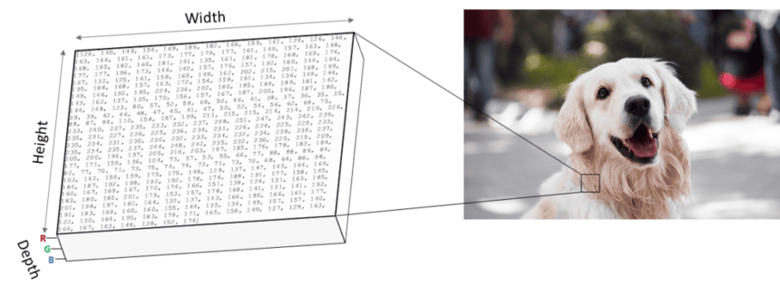
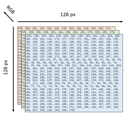
A digital image is a three-dimensional array of integer values. One dimension of this array represents the pixel width, and one dimension represents the height of the picture. The third dimension contains the color depth, defined by the image format. As shown below, we can thus represent the format of a digital image as “width x height x depth.” Next, let’s have a quick look at different image formats.

Overview of Different Image Formats

We can train CNNs with different image formats, but the input data are always multidimensional arrays of integer values. One of the most commonly used color formats in deep learning is “RGB.” RGB stands for the three color channels: “Red,” “Green,” and “Blue.” RGB images are divided into three layers of integer values, one layer for each color channel—the integer values of a 16-bit RGB image in each layer range from 1 to 255. Together, the three layers can reproduce 65,536 different colors.

In contrast to RGB images, grey-scale images only have a single color layer. This layer resembles the brightness of each pixel in the image. Consequently, the format of a grey-scale image is width x height x 1. Using grey-scale images or images with black and white shades instead of RGB images can speed up the training process because less data needs to be processed. However, image data with multiple color channels provide the model with more information, leading to better predictions. The RGB format is often a good choice between prediction quality and performance. Next, let’s look at how CNNs handle digital images in the learning process.

Convolutional Neural Networks

As mentioned before, a CNN is a specific form of an artificial neural network. The main difference between the CNN and the standard multi-layer perceptron is their convolutional layers. CNNs can have other layers, but the convolutions make a CNN so good at detecting objects. They allow the network to identify patterns based on features that work regardless of where in the image they occur. Let’s see how this works in more detail.

Convolutional Layers

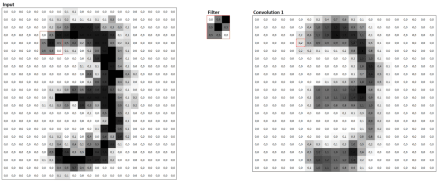
Convolutional layers use a rasterizing technique that breaks down an image into smaller groups of pixels called filters. Filters act as feature detectors from the original image. The primary purpose is to extract meaningful features from the input images.

During the training, the CNN slides the filter over image locations and calculates the dot product for each feature at a time. The results of these calculations are stored in a so-called feature map (sometimes called an activation map). A feature map represents where in the image a particular feature was identified. Subsequently, the values from the feature map are transformed with an activation function (usually ReLu), and the algorithm uses them as input to the next layer.

Features become more complex with the increasing depth of the network. In the first layer of the network, convolutions will detect generic geometric forms and low-level features based on edges, corners, squares, or circles. The subsequent layers of the network will look at more sophisticated shapes and may, for example, include features that resemble the form of an eye of a cat or the nose of a dog. In this way, convolutions provide the network with features at different levels of detail that enable powerful detection patterns.

Pooling / Downsampling

A convolutional layer is usually followed by a pooling operation, which reduces the amount of data by filtering unnecessary information. This process is also called downsampling or subsampling. There are various forms of pooling. In the most common variant – max-pooling – only the highest value in a predefined grid (e.g., 2×2) is processed, and the remaining values are discarded. For example, imagine a 2×2 grid with values 0.1, 0.5, 0.4, and 0.8. The algorithm would only process the 0,8 further for this grid and use it as part of the input to the next layer. The advantages of pooling are reduced data and faster training times. Because pooling minimizes the complexity of the network, it allows for the construction of deeper architectures with more layers. In addition, pooling offers a certain protection against overfitting during training.

Dropout

Dropout is another technique that helps prevent the network from overfitting the training data. When we activate Dropout for a layer, the algorithm will remove a random number of neurons from the layer per training step. As a result, the network needs to learn patterns that give less weight to individual layers and thus generalize better. The dropout rate controls the percentage of switched-off neurons in each training iteration. We can configure Dropout for each layer separately.

CNNs with many layers and training epochs tend to overfit the training data. Especially here, Dropout is crucial to avoid overfitting and to achieve good prediction results with data that the network does not know yet. A typical value for the rate lies between 10% to 30%.

Multi-Layer Perceptron (MLP)

The CNN architecture ends with multiple dense layers that are fully connected. The layers are part of a Multilayer Perception (MLP), which has the task of dense down the results from the previous convolutions and outputting one of the multiple classes. Consequently, the number of neurons in the final dense layer usually corresponds to the number of different classes to be predicted. It is also possible to use a single neuron in the final layer for two-class prediction problems. In this case, the last neuron outputs a binary label of 0 or 1.

Building a CNN with Tensorflow that Classifies Cats and Dogs

Now that you are familiar with the basic concepts behind convolutional neural networks, we can commence with the practical part and build an image classifier. In the following, we will train a CNN to distinguish images of cats and dogs. We first define a CNN model and then feed it a few thousand photos from a public dataset with labeled images of cats and dogs.

Distinguishing cats and dogs may not sound difficult, but many challenges exist. Imagine the almost infinite circumstances in which animals can be photographed, not to mention the many forms a cat can take. These variations lead to the fact that even humans sometimes confuse a cat with a dog or vice versa. So don’t expect our model to be perfect right from the start. Our model will score around 82% accuracy on the validation dataset.

The code is available on the GitHub repository.

View on GitHub Relataly GitHub Repo

Prerequisites

Before starting the coding part, make sure that you have set up your Python 3 environment and required packages. If you don’t have an environment, you can follow this tutorial to set up the Anaconda environment.

Also, make sure you install all required packages. In this tutorial, we will be working with the following standard packages: 

• pandas
• NumPy
• math
• matplotlib

In addition, we will be using Keras (2.0 or higher) with Tensorflow backend and the machine learning library Scikit-learn.

You can install packages using console commands:

• pip install <package name>
• conda install <package name> (if you are using the anaconda packet manager)

Download the Dataset

We will train our image classification model with a public dataset from Kaggle.com. The dataset contains more than 25.000 JPG pictures of cats and dogs. The images are uniformly named and numbered, for example, dog.1.jpg, dog.2.jpg, dog.3.jpg, cat.1.jpg, cat.2.jpg, and so on. You can download the picture set directly from Kaggle: cats-vs-dogs.

Setup the Folder Structure

There are different ways data can be structured and loaded during model training. One approach (1) is to split the images into classes and create a separate folder for each class, class_a, class_b, etc. Another method (2) is to put all images into a single folder and define a DataFrame that splits the data into test and train. Because the cats and dogs dataset files already contain the classes in their name, I decided to go for the second approach.

Before we begin with the coding part, we create a folder structure that looks as follows:

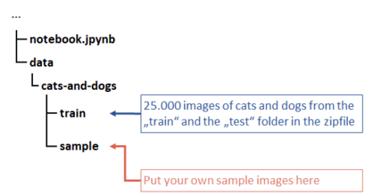
If you want to use the standard pathways given in the python tutorial, make sure that your notebook resides in the parent folder of the “data” folder.

After you have created the folder structure, open the cats-vs-dogs zip file. The ZIP file contains the folders “train,” “test,” and “sample.” Unzip the JPG files from the “train” (20.000 images) and the “test” folder (5.000 pictures) to the “train” folder of your project. Afterward, the train folder should contain 25.000 images. The sample folder is intended to include your sample images, for example, of your pet. We will later use the images from the sample folder to test the model on new real-world data.

We have fulfilled all requirements and can start with the coding part.

Step #1 Make Imports and Check Training Device

We begin by setting up the imports for this project. I have put the package imports at the beginning to give you a quick overview of the packages you need to install.

Using the GPU instead of the CPU allows for faster training times. However, setting up Tensorflow to work with the GPUs can cause problems. Not everyone has a GPU; in this case, TensorFlow should usually automatically run all code on the CPU. However, should you for any reason prefer to manually switch to CPU training, change [“CUDA_VISIBLE_DEVICES”]= “1” to “-1”. As a result, Tensorflow will run all code on the CPU and ignore all available GPUs.

import os
#os.environ["CUDA_VISIBLE_DEVICES"]="-1" 

import tensorflow as tf
from tensorflow.keras.preprocessing.image import ImageDataGenerator, array_to_img, img_to_array, load_img
from tensorflow.keras import Sequential
from tensorflow.keras.layers import Convolution2D, MaxPooling2D, ZeroPadding2D
from tensorflow.keras.layers import Conv2D, Activation, Dropout, Flatten, Dense, BatchNormalization
from tensorflow.keras.callbacks import EarlyStopping, ReduceLROnPlateau
from tensorflow.keras.metrics import Accuracy
from tensorflow.keras import regularizers
from tensorflow.keras.optimizers import SGD, Adam
from tensorflow.python.client import device_lib
from sklearn.model_selection import train_test_split
from sklearn.metrics import confusion_matrix, accuracy_score

tf.config.allow_growth = True
tf.config.per_process_gpu_memory_fraction = 0.9

from random import randint
import seaborn as sns
import pandas as pd
import numpy as np
import matplotlib.pyplot as plt
import matplotlib.colors as mcolors
import seaborn as sns
from PIL import Image
import random as rdn

Running the command below checks the TensorFlow version and the number of available GPUs in our system.

# check the tensorflow version
print('Tensorflow Version: ' + tf.__version__)

# check the number of available GPUs
physical_devices = tf.config.list_physical_devices('GPU')
print("Num GPUs:", len(physical_devices))

Tensorflow Version: 2.4.0-rc3
Num GPUs: 1

My GPU is an RTX 3080. When I wrote this article, the GPU was not yet supported by the standard TensorFlow release. I have therefore used the pre-release version of TensorFlow (2.4.0-rc3). I expect the following standard release (2.3) to work fine.

In my case, the GPU check returns one because I have a single GPU on my computer. If TensorFlow doesn’t recognize any GPU, this command will return 0. Tensorflow will then run on the CPU.

Step #2 Define the Prediction Classes

Next, we will define the path to the folders that contain our train and validation images. In addition, we will define a Dataframe “image_df,” which has all the pictures from the “train” folder. With the help of this Dataframe, we can later split the data simply by defining which images from the train folder contain the training dataset and which belong to the test dataset. Important note: the dataframe “image_df” only includes the names of the images and the classes, but not the photos themselves.

It’s good to check the distribution of classes in the training data set. For this purpose, we create a bar plot, which illustrates the number of both classes in the image data. And yes, I admit, I choose some custom colors to make it look fancy.

# set the directory for train and validation images
train_path = 'data/images/cats-and-dogs/train/'
#test_path = 'data/cats-and-dogs/test/'

# function to create a list of image labels 
def createImageDf(path):
    filenames = os.listdir(path)
    categories = []

    for fname in filenames:
        category = fname.split('.')[0]
        if category == 'dog':
            categories.append(1)
        else:
            categories.append(0)
    df = pd.DataFrame({
        'filename':filenames,
        'category':categories
    })
    return df

# display the header of the train_df dataset
image_df = createImageDf(train_path)
image_df.head(5)

sns.countplot(y='category', data=image_df, palette=['#2FE5C7',"#2F8AE5"], orient="h")

The number of images in the two classes is balanced, so we don’t need to rebalance the data. That’s nice!

Step #3 Plot Sample Images

I prefer not to jump directly into preprocessing and check that the data has been correctly loaded. We will do this by plotting some random images from the train folder. This step is not necessary, but it’s a best practice.

n_pictures = 16 # number of pictures to be shown
columns = int(n_pictures / 2)
rows = 2
plt.figure(figsize=(40, 12))
for i in range(n_pictures):
    num = i + 1
    ax = plt.subplot(rows, columns, i + 1)
    if i < columns:
        image_name = 'cat.' + str(rdn.randint(1, 1000)) + '.jpg'
    else: 
        image_name = 'dog.' + str(rdn.randint(1, 1000)) + '.jpg'
    plt.xlabel(image_name)    
    plt.imshow(load_img(train_path + image_name)) 

#if you get a deprecated warning, you can ignore it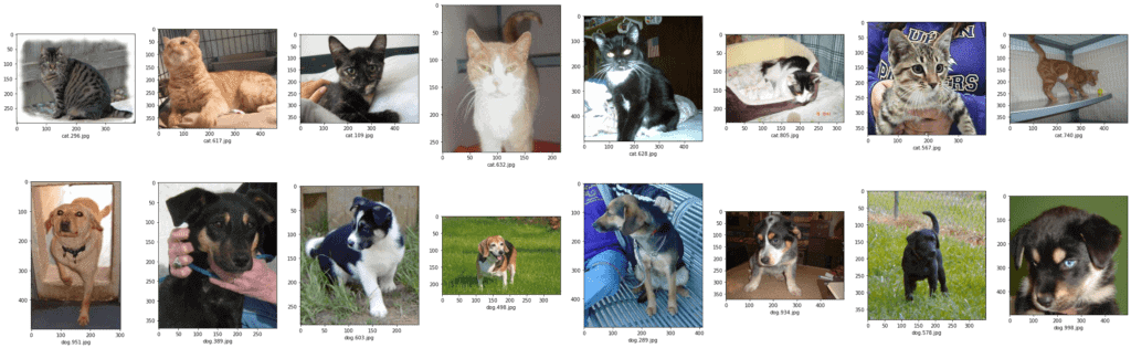

I never expected to have so many pictures of cats and dogs one day, but I guess neither did you 🙂 Neural networks require a fixed input shape where each neuron corresponds to a pixel value.

As we can see from the sample images, the images in our dataset have different sizes and aspect ratios. For the images to fit into the input shape of our neural network, we need to put the images into a standard format. But before that, we split the data into two datasets for train and test.

Step #4 Split the Data

Image classification requires splitting the data into a train and a validation set. We define a split ratio of 1/5 so that 80% of the data goes into the training dataset and 20% goes into the validation dataframe. We shuffle the data to create two DataFrameswith a mix of random cat and dog pictures. In addition, we transform the classes of the images into categorical values 0->”cat” and 1->”dog”. The result is two new DataFrames: train_df (20.000 images) and validate_df (5.000 images).

image_df["category"] = image_df["category"].replace({0:'cat',1:'dog'})

train_df, validate_df = train_test_split(image_df, test_size=0.20, random_state=42)
train_df = train_df.reset_index(drop=True)
total_train = train_df.shape[0]

validate_df = validate_df.reset_index(drop=True)
total_validate = validate_df.shape[0]
train_df.head()

print(len(train_df), len(validate_df))

Output: 20000 5000

Step #5 Preprocess the Images

The next step is to define two data generators for these DataFrames, which use the names given in the train and validation DataFrames to feed the images from the “train” path into our neural network. The data generator has various configuration options. We will perform the following operations:

• Rescale the image by dividing their RGB color values (1-255) by 255
• Shuffle the images (again)
• Bring the images into a uniform shape of 128 x 128 pixels
• We define a batch size of 32, which processes the 32 images simultaneously.
• The class mode is “binary” so our two prediction labels are encoded as float32 scalars with values 0 or 1. As a result, we will only have a single end neuron in our network.
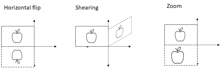
• We perform some data augmentation techniques on the training data (incl. horizontal flip, shearing, and zoom). In this way, the model never sees different variants of the images, which helps to prevent overfitting.

It is essential to mention that the input shape of the first layer of the neural network must correspond to the image shape of 128 x 128. The reason is that each pixel becomes an input to a neuron.

# set the dimensions to which we will convert the images
img_width, img_height = 128, 128
target_size = (img_width, img_height)
batch_size = 32
rescale=1.0/255

# configure the train data generator
print('Train data:')
train_datagen = ImageDataGenerator(rescale=rescale)
train_generator = train_datagen.flow_from_dataframe(
    train_df, 
    train_path,
    shear_range=0.2, #
    zoom_range=0.2, #
    horizontal_flip=True, # 
    shuffle=True, # shuffle the image data
    x_col='filename', y_col='category',
    classes=['dog', 'cat'],
    target_size=target_size,
    batch_size=batch_size,
    color_mode="rgb",
    class_mode='binary')

# configure test data generator
# only rescaling
print('Test data:')
validation_datagen = ImageDataGenerator(rescale=rescale)
validation_generator = validation_datagen.flow_from_dataframe(
    validate_df, 
    train_path,    
    shuffle=True,
    x_col='filename', y_col='category',
    classes=['dog', 'cat'],
    target_size=target_size,
    batch_size=batch_size,
    color_mode="rgb",
    class_mode='binary')

Train data:
Found 20000 validated image filenames belonging to 2 classes.
Test data:
Found 5000 validated image filenames belonging to 2 classes.

At this point, we have already completed the data preprocessing part. The next step is to define and compile the convolutional neural network.

Step #6 Define and Compile the Convolutional Neural Network

The architecture of our image classification CNN is inspired by the famous VGGNet. In this section, we will define and compile our CNN model. We do this by defining multiple layers and stacking them on top of each other. However, to lower the amount of time needed to train the network, I reduced the number of layers.

The initial layer of our network is the initial input layer, which receives the preprocessed images. As already noted, the shape of the input layer needs to match the shape of our images. Considering how we have defined the format of the images in our data generators, the input shape is defined as 128 x 128 x 3.

The subsequent layers are four convolutional layers. Each of these layers is followed by a pooling layer. In addition, we define a Dropoutrate of 20% for each convolutional layer.

Finally, a fully connected output layer with 128 neurons and a binary layer for the output complete the structure of the CNN.

# define the input format of the model
input_shape = (img_width, img_height, 3)
print(input_shape)

# define  model
model = Sequential()
model.add(Conv2D(32, (3, 3), strides=(1, 1), activation='relu', kernel_initializer='he_uniform', padding='same', input_shape=input_shape))
model.add(MaxPooling2D((2, 2)))
model.add(Dropout(0.20))
model.add(Conv2D(64, (3, 3), strides=(1, 1), activation='relu', kernel_initializer='he_uniform', padding='same'))
model.add(MaxPooling2D((2, 2)))
model.add(Dropout(0.20))
model.add(Conv2D(64, (3, 3), strides=(1, 1), activation='relu', kernel_initializer='he_uniform', padding='same'))
model.add(MaxPooling2D((2, 2)))
model.add(Dropout(0.20))
model.add(Conv2D(128, (3, 3),  strides=(1, 1),activation='relu', kernel_initializer='he_uniform', padding='same'))
model.add(MaxPooling2D((2, 2)))
model.add(Dropout(0.20))
model.add(Flatten())
model.add(Dense(128, activation='relu', kernel_initializer='he_uniform'))
model.add(Dropout(0.5))
model.add(Dense(1, activation='sigmoid'))

# compile the model and print its architecture
opt = SGD(lr=0.001, momentum=0.9)
history = model.compile(optimizer=opt, loss='binary_crossentropy', metrics=['accuracy'])
print(model.summary())

input_shape: (100, 100, 3)
Model: "sequential"
_________________________________________________________________
Layer (type)                 Output Shape              Param #   
=================================================================
conv2d (Conv2D)              (None, 100, 100, 32)      896       
_________________________________________________________________
max_pooling2d (MaxPooling2D) (None, 50, 50, 32)        0         
_________________________________________________________________
dropout (Dropout)            (None, 50, 50, 32)        0         
_________________________________________________________________
conv2d_1 (Conv2D)            (None, 50, 50, 64)        18496     
_________________________________________________________________
max_pooling2d_1 (MaxPooling2 (None, 25, 25, 64)        0         
_________________________________________________________________
dropout_1 (Dropout)          (None, 25, 25, 64)        0         
_________________________________________________________________
conv2d_2 (Conv2D)            (None, 25, 25, 64)        36928     
_________________________________________________________________
max_pooling2d_2 (MaxPooling2 (None, 12, 12, 64)        0         
_________________________________________________________________
dropout_2 (Dropout)          (None, 12, 12, 64)        0         
_________________________________________________________________
conv2d_3 (Conv2D)            (None, 12, 12, 128)       73856     
_________________________________________________________________
...
Trainable params: 720,257
Non-trainable params: 0
_________________________________________________________________
None

At this point, we have defined and assembled our convolutional neural network. Next, it is time to train the model.

Step #7 Train the Model

Before we train the image classifier, we still have to choose the number of epochs. More epochs can improve the model performance and lead to longer training times. In addition, the risk increases that the model overfits. Finding the optimal number of epochs is difficult and often requires a trial-and-error approach. I typically start with a small number of 5 epochs and then increase this number until increases do not lead to significant improvements.

# train the model
epochs = 40
early_stop = EarlyStopping(monitor='loss', patience=6, verbose=1)

history = model.fit(
    train_generator,
    epochs=epochs,
    callbacks=[early_stop],
    steps_per_epoch=len(train_generator),
    verbose=1,
    validation_data=validation_generator,
    validation_steps=len(validation_generator))

Epoch 1/35
625/625 [==============================] - 121s 194ms/step - loss: 0.7050 - accuracy: 0.5282 - val_loss: 0.6902 - val_accuracy: 0.5824
Epoch 2/35
625/625 [==============================] - 115s 183ms/step - loss: 0.6853 - accuracy: 0.5469 - val_loss: 0.6856 - val_accuracy: 0.5806
Epoch 3/35
625/625 [==============================] - 115s 184ms/step - loss: 0.6744 - accuracy: 0.5752 - val_loss: 0.6746 - val_accuracy: 0.5806
Epoch 4/35
625/625 [==============================] - 112s 180ms/step - loss: 0.6569 - accuracy: 0.5987 - val_loss: 0.6593 - val_accuracy: 0.6110
Epoch 5/35
625/625 [==============================] - 115s 185ms/step - loss: 0.6423 - accuracy: 0.6194 - val_loss: 0.6474 - val_accuracy: 0.6134
Epoch 6/35
625/625 [==============================] - 116s 185ms/step - loss: 0.6309 - accuracy: 0.6370 - val_loss: 0.6386 - val_accuracy: 0.6260
Epoch 7/35
625/625 [==============================] - 115s 183ms/step - loss: 0.6139 - accuracy: 0.6539 - val_loss: 0.6082 - val_accuracy: 0.6682

A quick comment on the required time to train the model. Although the model is not overly complex and the size of the data is still moderate, training the model can take some time. I made two training runs – the first run on my GPU (Nvidia Geforce 3080 RTX) and the second on my CPU (AMD Ryzen 3700x). On the GPU, training took approximately 10 minutes. The CPU training was much slower and took about 30 minutes, three times longer than the GPU.

After training, you may want to save the classification model and load it at a later time. You can do this with the code below:
However, we need to define the model strictly as it was during training before loading.

# Safe the weights
model.save_weights('cats-and-dogs-weights-v1.h5')

# Define model as during training
# model architecture

# Loads the weights
model.load_weights('cats-and-dogs-weights-v1.h5')

Step #8 Visualize Model Performance

After training the model, we want to check the performance of our image classification model. For this purpose, we can apply the same performance measures as in traditional classification projects. The code below illustrates the performance of our image classifier on the validation dataset.

To learn more about measuring model performance, check out my previous post on Measuring Model Performance.

def plot_loss(history, value1, value2, title):
    fig, ax = plt.subplots(figsize=(15, 5), sharex=True)
    plt.plot(history.history[value1], 'b')
    plt.plot(history.history[value2], 'r')
    plt.title(title)
    plt.ylabel("Loss")
    plt.xlabel("Epoch")
    ax.xaxis.set_major_locator(plt.MaxNLocator(epochs))
    plt.legend(["Train", "Validation"], loc="upper left")
    plt.grid()
    plt.show()

# plot training & validation loss values
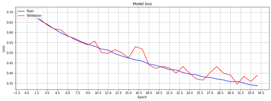
plot_loss(history, "loss", "val_loss", "Model loss")
# plot training & validation loss values
plot_loss(history, "accuracy", "val_accuracy", "Model accuracy")

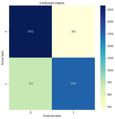
Next, let’s print the accuracy and a confusion matrix on the predictions from the validation dataset.

# function that returns the label for a given probability
def getLabel(prob):
    if(prob > .5):
               return 'dog'
    else:
               return 'cat'

# get the predictions for the validation data
val_df = validate_df.copy()
val_df['pred'] = ""
val_pred_prob = model.predict(validation_generator)

for i in range(val_pred_prob.shape[0]):
    val_df['pred'][i] = getLabel(val_pred_prob[i])
          
# create a confusion matrix
y_val = val_df['category']
y_pred = val_df['pred']

print('Accuracy: {:.2f}'.format(accuracy_score(y_val, y_pred)))
cnf_matrix = confusion_matrix(y_val, y_pred)

# plot the confusion matrix in form of a heatmap

%matplotlib inline
class_names=[False, True] # name  of classes
fig, ax = plt.subplots(figsize=(8, 8))
tick_marks = np.arange(len(class_names))
plt.xticks(tick_marks, class_names)
plt.yticks(tick_marks, class_names)
sns.heatmap(pd.DataFrame(cnf_matrix), annot=True, cmap="YlGnBu", fmt='g')
plt.title('Confusion matrix')
plt.ylabel('Actual label')
plt.xlabel('Predicted label')

Accuracy: 0.82

Step #9 Image Classification on Sample Images

Now that we have trained the model, I bet you can’t wait to test the image classifier on some sample data. For this purpose, ensure that you have some sample images in the “sample” folder. Running the code below will feed the image classifier with the test dataset. Based on this dataset, the model will then predict the labels for the images from the sample folder. Finally, the code below prints the images in an image grid and the predicted labels.

# set the path to the sample images
sample_path = "data/images/cats-and-dogs/sample/"
sample_df = createImageDf(sample_path)
sample_df['category'] = sample_df['category'].replace({0:'cat',1:'dog'})
sample_df['pred'] = ""

# create an image data generator for the sample images - we will only rescale the images
test_datagen = ImageDataGenerator(rescale=1./255)
test_generator = test_datagen.flow_from_dataframe(
    sample_df, 
    sample_path,    
    shuffle=False,
    x_col='filename', y_col='category',
    target_size=target_size)

# make the predictions 
pred_prob = model.predict(test_generator)
image_number = pred_prob.shape[0]

# define the plot size
for i in range(pred_prob.shape[0]):
    sample_df['pred'][i] = getLabel(pred_prob[i])
    
print('Accuracy: {:.2f}'.format(accuracy_score(sample_df['category'], sample_df['pred'])))

nrows = 6
ncols = int(round(image_number / nrows, 0))
fig, axs = plt.subplots(nrows, ncols, figsize=(15, 15))
for i, ax in enumerate(fig.axes):
    if i < sample_df.shape[0]:
        filepath = sample_path + sample_df.at[i ,'filename']
        ax = ax
        img = Image.open(filepath).resize(target_size)
        ax.imshow(img)
        ax.set_title(sample_df.at[i ,'filename'] + '\n' + ' predicted: '  + str(sample_df.at[i ,'pred']))
        result = [True if sample_df.at[i ,'pred'] == sample_df.at[i ,'category'] else False]
        ax.set_xlabel(str(result))
        ax.set_xticks([]); ax.set_yticks([])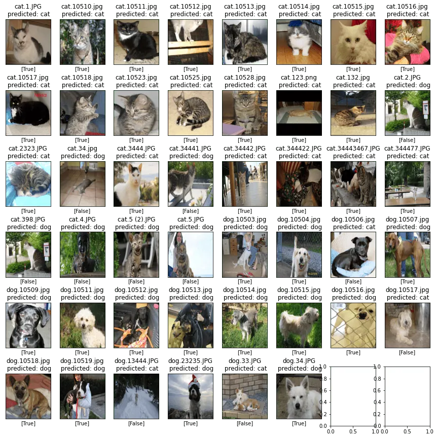

Our image classifier achieves an accuracy of around 83% on the validation set. The model is not perfect, but it should have labeled most images correctly. With deeper architectures, more data, and training runs, you can create classification models that achieve better results over 95%.

Summary

In this tutorial, you learned how to train an image classification model. We have prepared a dataset and performed several transformations to bring the data in shape for training. Finally, we have trained a convolutional neural network to distinguish between dogs and cats. You can now use this knowledge to train image classification models that determine other objects.

There are many other cool things that you can do with CNNs. For example, object localization in images and videos and even stock market prediction. But these are topics for further articles.

I am always happy to receive feedback. I hope you enjoyed the article and would be happy if you left a comment. Cheers

Sources and Further Reading

1. Andriy Burkov Machine Learning Engineering
2. Oliver Theobald (2020) Machine Learning For Absolute Beginners: A Plain English Introduction
3. Charu C. Aggarwal (2018) Neural Networks and Deep Learning
4. Aurélien Géron (2019) Hands-On Machine Learning with Scikit-Learn, Keras, and TensorFlow: Concepts, Tools, and Techniques to Build Intelligent Systems
5. David Forsyth (2019) Applied Machine Learning Springer
6. [1] D. H. Hubel and T. N. Wiesel – Receptive Fields of Neurons in the Cat’s Striate Cortex, The Journal of physiology (1959)

The links above to Amazon are affiliate links. By buying through these links, you support the Relataly.com blog and help to cover the hosting costs. Using the links does not affect the price.