

Perfecting your machine learning model’s hyperparameters can often feel like hunting for a proverbial needle in a haystack. But with the Random Search algorithm, this intricate process of hyperparameter tuning can be efficiently automated, saving you valuable time and effort. Hyperparameters are properties intrinsic to your model, like the number of estimators in an ensemble model, and heavily influence its performance. Unlike model parameters, which are discovered during training by the machine learning algorithm, hyperparameters require pre-specification.
In this comprehensive Python tutorial, we’ll guide you on how to harness the power of Random Search to optimize a regression model’s hyperparameters. Our illustrative example utilizes a Support Vector Machine (SVM) for predicting house prices. However, the fundamental principles you’ll learn can be seamlessly applied to any model. So why painstakingly fine-tune hyperparameters manually when Random Search can handle the task efficiently?
Here’s a preview of what this Python tutorial entails:
- A brief overview of how Random Search operates and instances where it might be preferable to Grid Search.
- A hands-on Python tutorial featuring a public house price dataset from Kaggle.com. The aim here is to train a regression model capable of predicting US house prices based on various properties.
- Training a ‘best-guess’ model in Python, followed by using Random Search to discover a model with enhanced performance.
- Finally, we’ll implement cross-validation to validate our models’ performance.
By the end of this tutorial, you’ll be well-equipped to let Random Search efficiently fine-tune your model’s hyperparameters, freeing up your time for other crucial tasks.
Hyperparameter Tuning
Hyperparameters are configuration options that allow us to customize machine learning models and improve their performance. While normal parameters are the internal coefficients that the model learns during training, we need to specify hyperparameters before the training. It is usually impossible to find the best configuration without testing different configurations.
Searching for a suitable model configuration is called “hyperparameter tuning” or “hyperparameter optimization.” Machine learning algorithms have varying hyperparameters and parameter values. For example, a random decision forest classifier allows us to configure varying parameters such as the number of trees, the maximum tree depth, and the minimum number of nodes required for a new branch.
The hyperparameters and the range of possible parameter values span a search space in which we seek to identify the best configuration. The larger the search space, the more difficult it gets to find an optimal model. We can use random search to automatize this process.

Techniques for Tuning Hyperparameters
Hyperparameter tuning is the process of adjusting the hyperparameters of a machine learning algorithm to optimize its performance on a specific dataset or task. Several techniques can be used for hyperparameter tuning, including:
- Grid Search: grid search is a brute-force search algorithm that systematically evaluates a given set of hyperparameter values by training and evaluating a model for each combination of values. It is a simple and effective technique, but it can be computationally expensive, especially for large or complex datasets.
- Random Search: As mentioned, random search is an alternative to grid search that randomly samples a given set of hyperparameter values rather than evaluating all possible combinations. It can be more efficient than grid search, but it may not find the optimal set of hyperparameters.
- Bayesian Optimization: A bayesian optimization is a probabilistic approach to hyperparameter tuning, which uses Bayesian inference to model the distribution of hyperparameter values that are likely to produce a good performance. It can be more efficient and effective than grid search or random search, but it can be more challenging to implement and interpret.
- Genetic Algorithms: genetic algorithms are optimization algorithms inspired by the principles of natural selection and genetics. They use a population of candidate solutions, which are iteratively evolved and selected based on their fitness or performance, to find the optimal set of hyperparameters.
In this article, we specifically look at the Random Search technique.

What is Random Search?
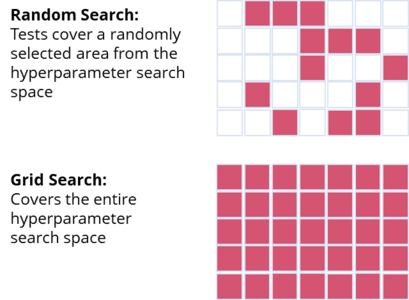
The random search algorithm generates models from hyperparameter permutations randomly selected from a grid of parameter values. The idea behind the randomized approach is that testing random configurations efficiently identifies a good model. We can use random search both for regression and classification models.
Random Search and Grid Search are the most popular techniques for hyperparametric tuning, and both methods are often compared. Unlike random search, grid search covers the search space exhaustively by trying all possible variants. The technique works well for testing a small number of configurations already known to work well.
As long as both search space and training time are small, the grid search technique is excellent for finding the best model. However, the number of model variants increases exponentially with the size of the search space. It is often more efficient for large search spaces or complex models to use random search.
Since random search does not exhaustively cover the search space, it does not necessarily yield the best model. However, it is also much faster than grid search and efficient in delivering a suitable model in a short time.
Tuning the Hyperparameters of a Random Decision Forest Regressor in Python using Random Search
In this tutorial, we delve into the use of the Random Search algorithm in Python, specifically for predicting house prices. We’ll be using a dataset rich in diverse house characteristics. Various elements, such as data quality and quantity, model intricacy, the selection of machine learning algorithms, and housing market stability, significantly influence the accuracy of house price predictions.
Our initial model employs a Random Decision Forest algorithm, which we’ll optimize using a random search approach for hyperparameters tuning. By identifying and implementing a more advantageous configuration, we aim to enhance our model’s performance significantly.
Here’s a concise outline of the steps we’ll undertake:
- Loading the house price dataset
- Exploring the dataset intricacies
- Preparing the data for modeling
- Training a baseline Random Decision Forest model
- Implementing a random search approach for model optimization
- Measuring and evaluating the performance of our optimized model
Through this step-by-step guide, you’ll learn to enhance model performance, further refining your understanding of Random Search algorithm implementation in Python.
The Python code is available in the relataly GitHub repository.

Prerequisites
Before starting the coding part, ensure that you have set up your Python (3.8 or higher) environment and required packages. If you don’t have an environment, follow this tutorial to set up the Anaconda environment.
Also, make sure you install all required packages. In this tutorial, we will be working with the following standard packages:
In addition, we will be using the Python Machine Learning library Scikit-learn to implement the random forest and the grid search technique.
You can install packages using console commands:
- pip install <package name>
- conda install <package name> (if you are using the anaconda packet manager)
House Price Prediction: About the Use Case and the Data
House price prediction is the process of using statistical and machine learning techniques to predict the future value of a house. This can be useful for a variety of applications, such as helping homeowners and real estate professionals to make informed decisions about buying and selling properties. In order to make accurate predictions, it is important to have access to high-quality data about the housing market.
In this tutorial, we will work with a house price dataset from the house price regression challenge on Kaggle.com. The dataset is available via a git hub repository. It contains information about 4800 houses sold between 2016 and 2020 in the US. The data includes the sale price and a list of 48 house characteristics, such as:
- Year – The year of construction,
- SaleYear – The year in which the house was sold
- Lot Area – The lot area of the house
- Quality – The overall quality of the house from one (lowest) to ten (highest)
- Road – The type of road, e.g., paved, etc.
- Utility – The type of the utility
- Park Lot Area – The parking space included with the property
- Room number – The number of rooms

Step #1 Load the Data
We begin by loading the house price data from the relataly GitHub repository. A separate download is not required.
# A tutorial for this file is available at www.relataly.com

import pandas as pd
import numpy as np
import matplotlib.pyplot as plt
import seaborn as sns
from sklearn.model_selection import RandomizedSearchCV, train_test_split
from sklearn.metrics import mean_absolute_error, mean_absolute_percentage_error
from sklearn import svm

# Source:
# https://www.kaggle.com/c/house-prices-advanced-regression-techniques

# Load train and test datasets
path = "https://raw.githubusercontent.com/flo7up/relataly_data/main/house_prices/train.csv"
df = pd.read_csv(path)
print(df.columns)
df.head()
Index(['Id', 'MSSubClass', 'MSZoning', 'LotFrontage', 'LotArea', 'Street',
       'Alley', 'LotShape', 'LandContour', 'Utilities', 'LotConfig',
       'LandSlope', 'Neighborhood', 'Condition1', 'Condition2', 'BldgType',
       'HouseStyle', 'OverallQual', 'OverallCond', 'YearBuilt', 'YearRemodAdd',
       'RoofStyle', 'RoofMatl', 'Exterior1st', 'Exterior2nd', 'MasVnrType',
       'MasVnrArea', 'ExterQual', 'ExterCond', 'Foundation', 'BsmtQual',
       'BsmtCond', 'BsmtExposure', 'BsmtFinType1', 'BsmtFinSF1',
       'BsmtFinType2', 'BsmtFinSF2', 'BsmtUnfSF', 'TotalBsmtSF', 'Heating',
       'HeatingQC', 'CentralAir', 'Electrical', '1stFlrSF', '2ndFlrSF',
       'LowQualFinSF', 'GrLivArea', 'BsmtFullBath', 'BsmtHalfBath', 'FullBath',
       'HalfBath', 'BedroomAbvGr', 'KitchenAbvGr', 'KitchenQual',
       'TotRmsAbvGrd', 'Functional', 'Fireplaces', 'FireplaceQu', 'GarageType',
       'GarageYrBlt', 'GarageFinish', 'GarageCars', 'GarageArea', 'GarageQual',
       'GarageCond', 'PavedDrive', 'WoodDeckSF', 'OpenPorchSF',
       'EnclosedPorch', '3SsnPorch', 'ScreenPorch', 'PoolArea', 'PoolQC',
       'Fence', 'MiscFeature', 'MiscVal', 'MoSold', 'YrSold', 'SaleType',
       'SaleCondition', 'SalePrice'],
      dtype='object')
	Id	MSSubClass	MSZoning	LotFrontage	LotArea	Street	Alley	LotShape	LandContour	Utilities	...	PoolArea	PoolQC	Fence	MiscFeature	MiscVal	MoSold	YrSold	SaleType	SaleCondition	SalePrice
0	1	60			RL			65.0		8450	Pave	NaN		Reg			Lvl			AllPub		...	0			NaN		NaN		NaN			0		2		2008	WD			Normal			208500
1	2	20			RL			80.0		9600	Pave	NaN		Reg			Lvl			AllPub		...	0			NaN		NaN		NaN			0		5		2007	WD			Normal			181500
2	3	60			RL			68.0		11250	Pave	NaN		IR1			Lvl			AllPub		...	0			NaN		NaN		NaN			0		9		2008	WD			Normal			223500
3	4	70			RL			60.0		9550	Pave	NaN		IR1			Lvl			AllPub		...	0			NaN		NaN		NaN			0		2		2006	WD			Abnorml			140000
4	5	60			RL			84.0		14260	Pave	NaN		IR1			Lvl			AllPub		...	0			NaN		NaN		NaN			0		12		2008	WD			Normal			250000
5 rows × 81 columns
Step #2 Explore the Data
Before jumping into preprocessing and model training, let’s quickly explore the data. A distribution plot can help us understand our dataset’s frequency of regression values.
# Create histograms for feature columns separated by prediction label value
ax = sns.displot(data=df[['SalePrice']].dropna(), height=6, aspect=2)
plt.title('Sale Price Distribution')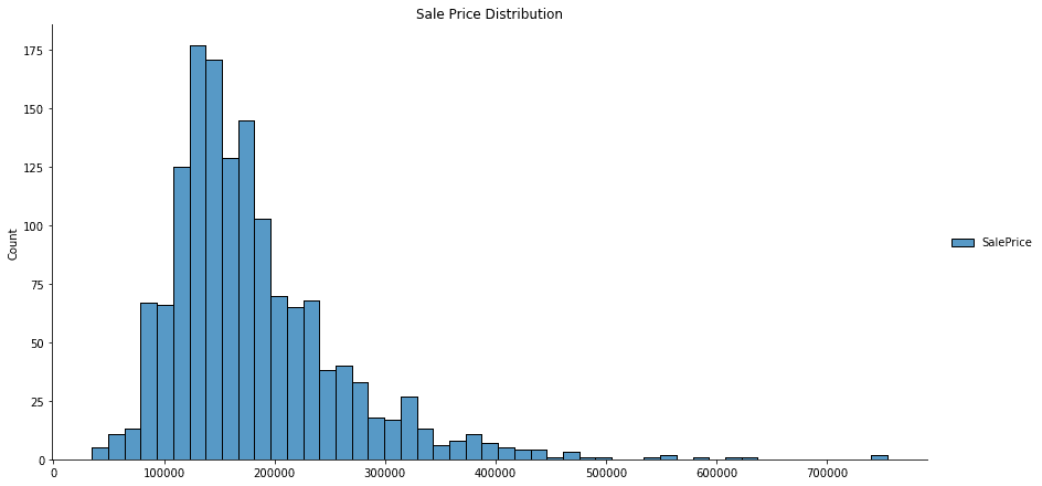
For feature selection, it is helpful to understand the predictive power of the different variables in a dataset. We can use scatterplots to estimate the predictive power of specific features. Running the code below will create a scatterplot that visualizes the relation between the sale price, lot area, and the house’s overall quality.
# Create histograms for feature columns separated by prediction label value
plt.figure(figsize=(16,6))
df_features = df[['SalePrice', 'LotArea', 'OverallQual']]
sns.scatterplot(data=df_features, x='LotArea', y='SalePrice', hue='OverallQual')
plt.title('Sale Price Distribution')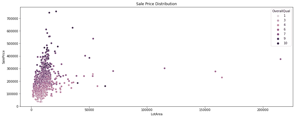
As expected, the scatterplot shows that the sale price increases with the overall quality. On the other hand, the LotArea has only a minor effect on the sale price.
Step #3 Data Preprocessing
Next, we prepare the data for use as input to train a regression model. Because we want to keep things simple, we reduce the number of variables and use only a small set of features. In addition, we encode categorical variables with integer dummy values.
To ensure that our regression model does not know the target variable, we separate house price (y) from features (x). Last, we split the data into separate datasets for training and testing. The result is four different data sets: x_train, y_train, x_test, and y_test.
def preprocessFeatures(df):
    # Define a list of relevant features
    feature_list = ['SalePrice', 'OverallQual', 'Utilities', 'GarageArea', 'LotArea', 'OverallCond']
    df_dummy = pd.get_dummies(df[feature_list])
    # Cleanse records with na values
    #df_prep = df_prep.dropna()
    return df_dummy

df_base = preprocessFeatures(df)

# Split the data into x_train and y_train data sets
x_train, x_test, y_train, y_test = train_test_split( df_base.copy(), df_base['SalePrice'].copy(), train_size=0.7, random_state=0)
x_train
OverallQual GarageArea LotArea OverallCond Utilities_AllPub Utilities_NoSeWa 682 6 431 2887 5 1 0 960 5 0 7207 7 1 0 1384 6 280 9060 5 1 0 1100 2 246 8400 5 1 0 416 6 440 7844 7 1 0
Step #4 Train Different Regression Models using Random Search
Now that the dataset is ready, we can train the random decision forest regressor. To do this, we first define a dictionary with different parameter ranges. In addition, we need to define the number of model variants (n) that the algorithm should try. The random search algorithm then selects n random permutations from the grid and uses them to train the model.
We use the RandomSearchCV algorithm from the scikit-learn package. The “CV” in the function name stands for cross-validation. Cross-validation involves splitting the data into subsets (folds) and rotating them between training and validation runs. This way, each model is trained and tested multiple times on different data partitions. When the search algorithm finally evaluates the model configuration, it summarizes these results into a test score.
We use a Random Decision Forest – a robust machine learning algorithm that can handle classification and regression tasks. As a so-called ensemble model, the Random Forest considers predictions from a set of multiple independent estimators. The estimator is an important parameter to pass to the RandomSearchCV function. Random decision forests have several hyperparameters that we can use to influence their behavior. We define the following parameter ranges:
- max_leaf_nodes = [2, 3, 4, 5, 6, 7]
- min_samples_split = [5, 10, 20, 50]
- max_depth = [5,10,15,20]
- max_features = [3,4,5]
- n_estimators = [50, 100, 200]
These parameter ranges define the search space from which the randomized search algorithm (RandomSearchCV) will select random configurations. Other parameters will use default values as defined by scikit-learn.
# Define the Estimator and the Parameter Ranges
dt = RandomForestRegressor()
number_of_iterations = 20
max_leaf_nodes = [2, 3, 4, 5, 6, 7]
min_samples_split = [5, 10, 20, 50]
max_depth = [5,10,15,20]
max_features = [3,4,5]
n_estimators = [50, 100, 200]

# Define the param distribution dictionary
param_distributions = dict(max_leaf_nodes=max_leaf_nodes,
                           min_samples_split=min_samples_split,
                           max_depth=max_depth,
                           max_features=max_features,
                           n_estimators=n_estimators)

# Build the gridsearch
grid = RandomizedSearchCV(estimator=dt,
                          param_distributions=param_distributions,
                          n_iter=number_of_iterations,
                          cv = 5)

grid_results = grid.fit(x_train, y_train)

# Summarize the results in a readable format
print("Best params: {0}, using {1}".format(grid_results.cv_results_['mean_test_score'], grid_results.best_params_))
results_df = pd.DataFrame(grid_results.cv_results_)
Best params: [0.68738293 0.49581669 0.52138751 0.61235299 0.65360944 0.61165147
0.70392285 0.52278886 0.67687248 0.68219638 0.70031536 0.65842909
0.51939338 0.70801017 0.70911805 0.69543885 0.67983801 0.60744371
0.68270285 0.70741042], using {'n_estimators': 100, 'min_samples_split': 5, 'max_leaf_nodes': 7, 'max_features': 3, 'max_depth': 15}
mean_fit_time std_fit_time mean_score_time std_score_time param_n_estimators param_min_samples_split param_max_leaf_nodes param_max_features param_max_depth params split0_test_score split1_test_score split2_test_score split3_test_score split4_test_score mean_test_score std_test_score rank_test_score
0 0.049196 0.002071 0.004074 0.000820 50 20 5 4 15 {'n_estimators': 50, 'min_samples_split': 20, ... 0.662973 0.705533 0.669520 0.702608 0.696280 0.687383 0.017637 7
1 0.041115 0.000554 0.003046 0.000094 50 50 2 3 10 {'n_estimators': 50, 'min_samples_split': 50, ... 0.490984 0.527231 0.426270 0.523086 0.511513 0.495817 0.036978 20
2 0.043325 0.000779 0.003486 0.000447 50 50 2 5 20 {'n_estimators': 50, 'min_samples_split': 50, ... 0.484524 0.559358 0.485459 0.517253 0.560343 0.521388 0.033545 18
3 0.162083 0.005665 0.012420 0.004788 200 5 3 3 20 {'n_estimators': 200, 'min_samples_split': 5, ... 0.586586 0.638341 0.573437 0.626793 0.636608 0.612353 0.027021 14
4 0.166659 0.003026 0.010958 0.000084 200 10 4 3 15 {'n_estimators': 200, 'min_samples_split': 10,... 0.633305 0.679161 0.623236 0.661864 0.670481 0.653609 0.021636 13These are the five best models and their respective hyperparameter configurations.
Step #5 Select the best Model and Measure Performance
Finally, we will choose the best model from the list using the “best_model” function. We then calculate the MAE and the MAPE to understand how the model performs on the overall test dataset. We then print a comparison between actual sale prices and predicted sale prices.
# Select the best Model and Measure Performance
best_model = grid_results.best_estimator_
y_pred = best_model.predict(x_test)
y_df = pd.DataFrame(y_test)
y_df['PredictedPrice']=y_pred
y_df.head()
	SalePrice	PredictedPrice
529	200624		166037.831002
491	133000		135860.757958
459	110000		123030.336177
279	192000		206488.444327
655	88000		130453.604206
Next, let’s take a look at the classification errors.
# Mean Absolute Error (MAE)
MAE = mean_absolute_error(y_pred, y_test)
print('Mean Absolute Error (MAE): ' + str(np.round(MAE, 2)))

# Mean Absolute Percentage Error (MAPE)
MAPE = mean_absolute_percentage_error(y_pred, y_test)
print('Median Absolute Percentage Error (MAPE): ' + str(np.round(MAPE*100, 2)) + ' %')
Mean Absolute Error (MAE): 29591.56 Median Absolute Percentage Error (MAPE): 15.57 %
On average, the model deviates from the actual value by 16 %. Considering we only used a fraction of the available features and defined a small search space, there is much room for improvement.
Summary
This article has shown how we can use grid Search in Python to efficiently search for the optimal hyperparameter configuration of a machine learning model. In the conceptual part, you learned about hyperparameters and how to use random search to try out all permutations of a predefined parameter grid. The second part was a Python hands-on tutorial, in which you learned to use random search to tune the hyperparameters of a regression model. We worked with a house price dataset and trained a random decision forest regressor that predicts the sale price for houses depending on several characteristics. Then we defined parameter ranges and tested random permutations. In this way, we quickly identified a configuration that outperforms our initial baseline model.
Remember that a random search efficiently identifies a good-performing model but does not necessarily return the best-performing one. Tech random search techniques can be used to tune the hyperparameters of both regression and classification models.
Sources and Further Reading
I hope this article was helpful. If you have any questions or suggestions, please write them in the comments.
The links above to Amazon are affiliate links. By buying through these links, you support the Relataly.com blog and help to cover the hosting costs. Using the links does not affect the price.
