

Are you ready to learn about the exciting world of social media sentiment analysis using Python? In this article, we’ll dive into how companies are leveraging machine learning to extract insights from Twitter comments, and how you can do the same. By comparing two popular classification models – Naive Bayes and Logistic Regression – we’ll help you identify which one best fits your needs.
Businesses are using sentiment analysis to make better sense of the vast amounts of data available online and on social media platforms. Understanding customer opinions and feedback can help companies identify trends and make more informed decisions. Whether you’re a business professional looking to leverage the power of social media data or a machine learning enthusiast, this article has everything you need to get started.
We’ll begin with an introduction to the concept of sentiment analysis and its theoretical foundations. Then, we’ll guide you through the practical steps of implementing a sentiment classifier in Python. Our model will analyze text snippets and categorize them into one of three sentiment categories: “positive,” “neutral,” or “negative.” Finally, we’ll compare the performance of Naive Bayes and Logistic Regression classifiers.
By the end of this article, you’ll have the skills and knowledge to perform sentiment analysis on social media data and apply these insights to your business or personal projects. So let’s jump right in!

Also: Classifying Purchase Intention of Online Shoppers with Python
What is Sentiment Analysis?
Sentiment analysis is the process of identifying the sentiment, or emotional tone, of a piece of text. This can be useful for a wide range of applications, such as identifying customer sentiment towards a product or service, or detecting the overall sentiment of a social media post or news article.
Sentiment analysis is typically performed using natural language processing (NLP) techniques and machine learning algorithms. These tools allow computers to “understand” the meaning of text and identify the sentiment it contains. Sentiment analysis can be performed at various levels of granularity, from identifying the sentiment of an entire document to identifying the sentiment of individual words or phrases within a document.
How Sentiment Classification Works
There are many different approaches to sentiment analysis, and the specific methods used can vary depending on the specific application and the type of text being analyzed. Some common techniques for performing sentiment analysis include using machine learning algorithms to classify text as positive, negative, or neutral, and using lexicons, or lists of words with pre-defined sentiment, to identify the sentiment of individual words or phrases. In this way, it is possible to measure the emotions towards a specific topic, e.g., products, brands, political parties, services, or trends.
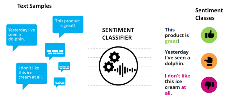
We can show how sentiment analysis works with a simple example:
- “This product is excellent!”
- “I don’t like this ice cream at all.”
- “Yesterday, I’ve seen a dolphin.”
While the first sentence denotes a positive sentiment, the second sentence is negative, and in the third sentence, the sentiment is neutral. A sentiment classifier can automatically label these sentences:
| Text Sequence | Sentiment Label |
| This product is great! | POSITIVE |
| I wouldn’t say I like this ice cream at all. | NEGATIVE |
| Yesterday I saw a dolphin. | NEUTRAL |
Predicting sentiment classes opens the door to more advanced statistical analysis and automated text processing.
Use Cases for Sentiment Analysis
Sentiment analysis is used in various application domains, including the following:
- Sentiment analysis can lead to more efficient customer service by prioritizing customer requests. For example, when customers complain about services or products, an algorithm can identify and prioritize these messages so that sales agents answer them first. This can increase customer satisfaction and reduce the churn rate.
- Twitter and Amazon reviews have become the first port of call for many customers today when exchanging information about products, brands, and trends or expressing their own opinions. A sentiment classifier systematically enables businesses to evaluate this information. It can collect data from social media posts and product reviews in real-time. For example, marketing managers can quickly obtain feedback on how well customers perceive campaigns and ads.
- In stock market prediction, analyze the sentiment of social media or news feeds towards stocks or brands. The sentiment is then used as an additional feature alongside price data to create better forecasting models. Some forecasting also approaches exclusively rely on sentiment.
Sentiment Analysis will find further adoption in the coming years. Especially in marketing and customer service, companies will increasingly use sentiment analysis to automate business processes and offer their customers a better customer experience.
How Sentiment Analysis Works: Feature Modelling
An essential step in the development of the Sentiment Classifier is language modeling. Before we can train a machine learning model, we need to bring the natural text into a structured format that the model can statistically assess in the training process. Various modeling techniques exist for this purpose. The two most common models are bag-of-words and n-grams.
Also: 9 Powerful Applications of OpenAI’s ChatGPT and Davinci
Bag-of-word Model
The bag-of-word model calculates probability distributions over the number of unique words. This approach converts individual words into individual features. Fill words with low predictive power, such as “the” or “a,” will be filtered out. Consider the following text sample:
“Bob likes to play basketball. But his friend Daniel prefers to play soccer. “
Through filtering of fill words, we convert his sample to:
“Bob”, “likes”, “play”, “basketball”, “friend”, “Daniel”, “play”, “soccer”.
In the next step, the algorithm converts these words into a normalized form, where each word becomes a column:
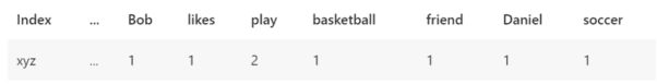
The bag-of-word model is easy to implement. However, it does not consider grammar or word order.
What is an N-gram Model?
The n-gram model considers multiple consecutive words in a text sequence and thus captures word sequence. The n stands for the number of words considered.
For example, in a 2-gram model, the sentence “Bob likes to play basketball. But his friend Daniel prefers to play soccer.” will be converted to the following model:
“Bob likes,” “likes to,” “to play,” “play basketball,” and so on. The n-gram model is often used to supplement the bag-of-word model. It is also possible to combine different n-gram models. For a 3-gram model, the text would be converted to “Bob likes to,” “likes to play,” “to play basketball,” and so on. Combining multiple n-gram models, however, can quickly increase model complexity.
Sentiment Classes and Model Training
The training of sentiment classifiers traditionally takes place in a supervised learning process. For this purpose, a training data set is used, which contains text sections with associated sentiment tendencies as prediction labels. Depending on which labels we provide and the training data, the classifier will learn to predict sentiment on a more or less fine-grained scale. Capturing neutral sentiment requires choosing an odd number of classes.
More advanced classifiers can detect different sorts of emotions and, for example, detect whether someone expresses anger, happiness, sadness, and so on. It basically comes down to which prediction labels you provide with the training data.
When the classifier is trained on a one-gram model, the classifier will learn that certain words such as “good” or “great” increase the probability that a text is associated with a positive sentiment. Consequently, when the classifier encounters these words in a new text sample, it will predict a higher probability of positive sentiment. On the other hand, the classifier will learn that words such as “hate” or “dislike” are often used to express negative opinions and thus increase the probability of negative sentiment.
Language Complications
Is sentiment analysis that simple? Well, not quite. The cases described so far were deliberately chosen to be very simple. However, human language is very complex, and many peculiarities make it more difficult in practice to identify the sentiment in a sentence or paragraph. Here are some examples:
- Inversions: “this product is not so great.”
- Typos: “I live this product!”
- Comparisons: “Product a is better than product z.”
- In a text passage, expression of pros and cons: “An advantage is that. But on the other hand…”
- Unknown vocabulary: “This product is just whuopii!”
- Missing words: “How can you not this product?”
Fortunately, there are methods to solve the complications mentioned above. I will explain more about them in one of my future articles. But for now, let’s stay with the basics and implement a simple classifier.
Training a Sentiment Classifier Using Twitter Data in Python
Venturing into the practical aspects of sentiment classification, our aim in this tutorial is to create an efficient sentiment classifier. Our focus will be on a dataset provided by Kaggle, comprising tens of thousands of tweets, each categorized as positive, neutral, or negative.
Our objective is to design a classifier capable of assigning one of these three sentiment categories to new text sequences. To this end, we will employ two distinct algorithms – Logistic Regression and Naive Bayes – as our estimators.
The tutorial culminates with a comparative analysis of the prediction performance of both models, followed by a set of test predictions. Through this hands-on approach, you will gain an understanding of the nuances of sentiment classification and its application in understanding public opinion, especially on social media platforms like Twitter.
Boost your sentiment analysis skills with our step-by-step guide, and learn to leverage machine learning tools for precise sentiment prediction.
The code is available on the GitHub repository.
Prerequisites
Before starting the coding part, make sure that you have set up your Python 3 environment and required packages. If you don’t have an environment, follow this tutorial to set up the Anaconda environment. Also, make sure you install all required packages. In this tutorial, we will be working with the following standard packages:
In addition, we will be using the machine learning libraries scikit-learn and seaborn for visualization.
You can install packages using console commands:
- pip install <package name>
- conda install <package name> (if you are using the anaconda packet manager)
About the Sentiment Dataset
Let’s begin with the technical part. First, we will download the data from the Twitter sentiment example on Kaggle.com. If you are working with the Kaggle Python environment, you can also directly save the data into your Python project.
We will only use the following two CSV files:
- train.csv: contains 27480 text samples.
- test.csv: contains 3533 text samples for validation purposes
The two files contain four columns:
- textID: An identifier
- text: The raw text
- selected_text: Contains a selected part of the original text
- sentiment: Contains the prediction label
We will copy the two files (train.csv and test.csv) into a folder that you can access from your Python environment. For simplicity, I recommend putting these files directly into the folder of your Python notebook. If you put them somewhere else, don’t forget to adjust the file path when loading the data.
Step #1 Load the Data
Assuming that you have copied the files into your Python environment, the next step is to load the data into your Python project and convert it into a Pandas DataFrame. The following code performs these steps and then prints a data summary.
import math
import numpy as np
import pandas as pd
import matplotlib.pyplot as plt
import matplotlib

from sklearn.pipeline import Pipeline
from sklearn.feature_extraction.text import CountVectorizer, TfidfTransformer
from sklearn.linear_model import LogisticRegression
from sklearn.naive_bayes import MultinomialNB
from sklearn.metrics import classification_report, multilabel_confusion_matrix
import scikitplot as skplt

import seaborn as sns

# Load the train data
train_path = "train.csv"
train_df = pd.read_csv(train_path)

# Load the test data
sub_test_path = "test.csv"
test_df = pd.read_csv(sub_test_path)

# Print a Summary of the data
print(train_df.shape, test_df.shape)
print(train_df.head(5))
			textID		text												selected_text									sentiment
0			cb774db0d1	I`d have responded, if I were going					I`d have responded, if I were going				neutral
1			549e992a42	Sooo SAD I will miss you here in San Diego!!!		Sooo SAD										negative
2			088c60f138	my boss is bullying me...							bullying me										negative
3			9642c003ef	what interview! leave me alone						leave me alone									negative
4			358bd9e861	Sons of ****, why couldn`t they put them on t...	Sons of ****,									negative
...
27481 rows × 4 columns
Step #2 Clean and Preprocess the Data
Next, let’s quickly clean and preprocess the data. First, as a best practice, we will transform the sentiment labels of the train and the test data into numeric values.
In addition, we will add a column in which we store the length of the text samples.
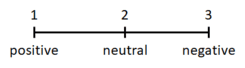
# Define Class Integer Values
cleanup_nums = {"sentiment": {"negative": 1, "neutral": 2, "positive": 3}}

# Replace the Classes with Integer Values
train_df = train_base_df.copy()
train_df.replace(cleanup_nums, inplace=True)

# Clean the Test Data
test_df = test_base_df.copy()
test_df.replace(cleanup_nums, inplace=True)

# Create a Feature based on Text Length
train_df['text_length'] = train_df['text'].str.len() # Store string length of each sample
train_df = train_df.sort_values(['text_length'], ascending=True)
train_df = train_df.dropna()
train_df
textID text selected_text sentiment text_length 14339 5c6abc28a1 ow ow 2 3.0 26005 0b3fe0ca78 ? ? 2 3.0 11524 4105b6a05d aw aw 2 3.0 641 5210cc55ae no no 2 3.0 25699 ee8ee67cb3 ME ME 2 3.0 ...
Step #3 Explore the Data
It’s always good to check the label distribution for a potential imbalance. We do this by plotting the distribution of labels in the text samples. This is important because it helps ensure that the trained model can make accurate predictions on new data. If the class labels are unbalanced, then the model is more likely to be biased toward the more common classes, which can lead to poor performance on less common classes.
Also: Feature Engineering and Selection for Regression Models
# Print the Distribution of Sentiment Labels
sns.set_theme(style="whitegrid")
ax = train_df['sentiment'].value_counts(sort=False).plot(kind='barh', color='b')
ax.set_xlabel('Count')
ax.set_ylabel('Labels')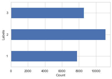
As we can see, our data is a bit imbalanced, but the differences are still within an acceptable range.
Let’s also quickly take a look at the distribution of text length.
# Visualize a distribution of text_length
sns.histplot(data=train_df, x='text_length', bins='auto', color='darkblue');
plt.title('Text Length Distribution')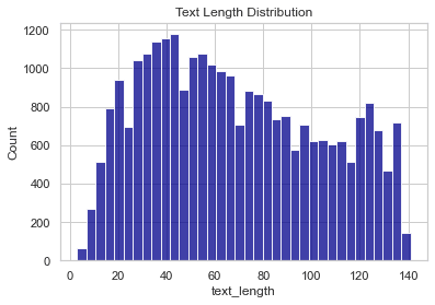
Step #4 Train a Sentiment Classifier
Next, we will prepare the data and train a classification model. We will use the pipeline class of the scikit-learn framework and a bag-of-word model to keep things simple. In NLP, we typically have to transform and split up the text into sentences and words. The pipeline class is thus instrumental in NLP because it allows us to perform multiple actions on the same data in a row.
The pipeline contains transformation activities and a prediction algorithm, the final estimator. In the following, we create two pipelines that use two different prediction algorithms:
- Logistic Regression
- Naive Bayes
4a) Sentiment Classification using Logistic Regression
The first model that we will train uses the logistic regression algorithm. We create a new pipeline. Then we add two transformers and the logistic regression estimator. The pipeline will perform the following activities.
- CountVectorizer: The vectorizer counts the number of words in each text sequence and creates the bag-of-word models.
- TfidfTransformer: The “Term Frequency Transformer” scales down the impact of words that occur very often in the training data and are thus less informative for the estimator than words that occur in a smaller fraction of the text samples. Examples are words such as “to” or “a.”
- Logistic Regression: By defining the multi_class as ‘auto,’ we will use logistic regression in a one-vs-all approach. This approach will split our three-class prediction problem into two two-class problems. Our model differentiates between one class and all other classes in the first step. Then all observations that do not fall into the first class enter a second model that predicts whether it is class two or three.
Our pipeline will transform the data and fit the logistic regression model to the training data. After executing the pipeline, we will directly evaluate the model’s performance. We will do this by defining a function that generates predictions on the test dataset and then evaluating the performance of our model. The function will print the performance results and store them in a dataframe. Later, when we want to compare the models, we can access the results from the dataframe.
# Create a transformation pipeline
# The pipeline sequentially applies a list of transforms and as a final estimator logistic regression
pipeline_log = Pipeline([
                ('count', CountVectorizer()),
                ('tfidf', TfidfTransformer()),
                ('clf', LogisticRegression(solver='liblinear', multi_class='auto')),
        ])

# Train model using the created sklearn pipeline
model_name = 'logistic regression classifier'
model_lgr = pipeline_log.fit(train_df['text'], train_df['sentiment'])

def evaluate_results(model, test_df):
    # Predict class labels using the learner function
    test_df['pred'] = model.predict(test_df['text'])
    y_true = test_df['sentiment']
    y_pred = test_df['pred']
    target_names = ['negative', 'neutral', 'positive']

    # Print the Confusion Matrix
    results_log = classification_report(y_true, y_pred, target_names=target_names, output_dict=True)
    results_df_log = pd.DataFrame(results_log).transpose()
    print(results_df_log)
    matrix = confusion_matrix(y_true,  y_pred)
    sns.heatmap(pd.DataFrame(matrix),
                annot=True, fmt="d", linewidths=.5, cmap="YlGnBu")
    plt.xlabel('Predictions')
    plt.xlabel('Actual')

    model_score = score(y_pred, y_true, average='macro')
    return model_score


# Evaluate model performance
model_score = evaluate_results(model_lgr, test_df)
performance_df = pd.DataFrame().append({'model_name': model_name,
                                    'f1_score': model_score[0],
                                    'precision': model_score[1],
                                    'recall': model_score[2]}, ignore_index=True)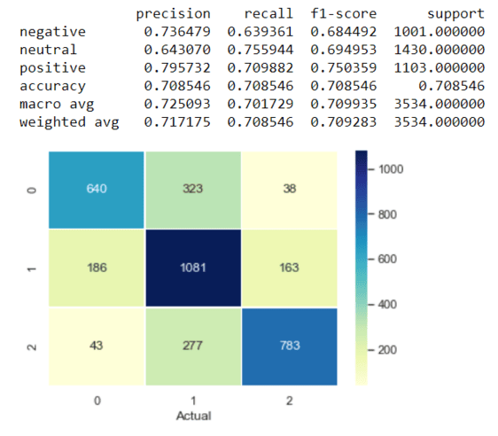
4b) Sentiment Classification using Naive Bayes
We will reuse the code from the last step to create another pipeline. However, we will exchange the Logistic Regressor with Naive Bayes (“MultinomialNB”). Naive Bayes is commonly used in natural language processing. The algorithm calculates the probability of each tag for a text sequence and then outputs the tag with the highest score. For example, the probabilities of the appearance of the words “likes” and “good” in texts within the category “positive sentiment” are higher than the probabilities of formation within the “negative” or “neutral” categories. In this way, the model predicts how likely it is for an unknown text that contains those words to be associated with either category.
We will reuse the previously defined function to print a classification report and plot the results in a confusion matrix.
# Create a pipeline which transforms phrases into normalized feature vectors and uses a bayes estimator
model_name = 'bayes classifier'

pipeline_bayes = Pipeline([
                ('count', CountVectorizer()),
                ('tfidf', TfidfTransformer()),
                ('gnb', MultinomialNB()),
                ])

# Train model using the created sklearn pipeline
model_bayes = pipeline_bayes.fit(train_df['text'], train_df['sentiment'])

# Evaluate model performance
model_score = evaluate_results(model_bayes, test_df)
performance_df = performance_df.append({'model_name': model_name,
                                    'f1_score': model_score[0],
                                    'precision': model_score[1],
                                    'recall': model_score[2]}, ignore_index=True)
Step #5 Measuring Multi-class Performance
So which classifier achieved better performance? It’s not so easy to say because it depends on the metrics. We will compare the classification performance of our two classifiers using the following metrics:
- Accuracy is calculated as the ratio between correctly predicted observations and total observations.
- Precision is calculated as the ratio between correctly labeled values and the sum of the correctly and incorrectly labeled positive observations.
- The formula for Recall is the ratio between correctly predicted observations and the sum of falsely classified observations.
- F1-Score takes all falsely labeled observations into account. It is, therefore, useful when you have an unequal class distribution.
You may wonder which of our three classes is the positive class. The answer is that we have to determine the positive class ourselves. By defining the positive class, we can consider that some classes may be more important than others. The other classes will then be counted as negative. You can see this in the confusion matrix in sections 5 and 6, containing separate metrics for each label.
Another option is to define a weighted average (see confusion matrix) that weights the quantity of the different labels in the overall dataset. For example, the negative label is weighted a bit higher than the neutral label because fewer observations with negative and positive labels are present in the data. Because our classes are equally important, I decided to use the weighted average.
Step #6 Comparing Model Performance
The following code calculates the performance metrics for the two classifiers and then creates a barplot to illustrate the results. In this specific case, the recall equals the accuracy.
If you want to learn more about measuring classification performance, check out this article.
# Compare model performance
print(performance_df)

performance_df = performance_df.sort_values('model_name')
fig, ax = plt.subplots(figsize=(12, 4))
tidy = performance_df.melt(id_vars='model_name').rename(columns=str.title)
sns.barplot(y='Model_Name', x='Value', hue='Variable', data=tidy, ax=ax, palette='husl',  linewidth=1, edgecolor="w")
plt.title('Model Outlier Detection Performance (Macro)')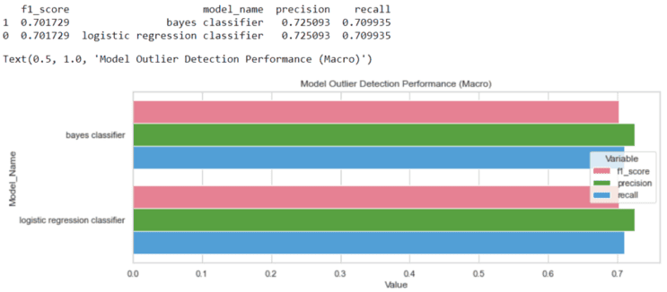
So we see that our Logistic Regression model performs slightly better than the Naive Bayes model. Of course, there are still many possibilities to improve the models further. In addition, there are several other methods and algorithms with which the performance could be significantly increased.
Step #7 Make Test Predictions
Finally, we use the Bayes classifier to generate some test predictions. Feel free to try it out! Change the text in the text phrases array and convince yourself that the classifier works.
testphrases = ['Mondays just suck!', 'I love this product', 'That is a tree', 'Terrible service']
for testphrase in testphrases:
    resultx = model_lgr.predict([testphrase]) # use model_bayes for predictions with the other model
    dict = {1: 'Negative', 2: 'Neutral', 3: 'Positive'}
print(testphrase + '-> ' + dict[resultx[0]])- Mondays suck!-> Negative
- I love this product-> Positive
- That is a tree-> Neutral
- Terrible service-> Negative
Summary
That’s it! In this tutorial, you have learned to build a simple sentiment classifier that can detect sentiment expressed through text on a three-class scale. We have trained and tested two standard classification algorithms – Logistic Regression and Naive Bayes. Finally, we have compared the performance of the two algorithms and made some test predictions.
The best way to deepen your knowledge of sentiment analysis is to apply it in practice. I thus want to encourage you to use your knowledge by tackling other NLP challenges. For example, you could build a sentiment classifier that assigns text phrases to labels such as sports, fashion, cars, technology, etc. If you are still looking for data you can use for such a project, you will find exciting ones on Kaggle.com.
Let me know if you found this tutorial helpful. I appreciate your feedback!
Sources and Further Reading
The links above to Amazon are affiliate links. By buying through these links, you support the Relataly.com blog and help to cover the hosting costs. Using the links does not affect the price.
