Rolling Time Series Forecasting: Creating a Multi-Step Prediction for a Rising Sine Curve using Neural Networks in Python

Many time forecasting problems can be solved by predicting just one step into the future. However, some problems require a forecast for an extended period of time, which calls for a multi-step time series forecasting approach. This approach involves modeling the distribution of future values of a signal over a prediction horizon. In this article, we use the rising sine curve as an example to demonstrate how to apply a multi-step prediction approach using Keras neural networks with LSTM layers in Python. We create a rolling forecast for the sine curve by generating several single-step predictions and iteratively using them as input to predict further steps in the future.
The remainder of this article proceeds as follows: We begin by looking at the sine curve problem and provide a quick intro to recurrent neural networks. After this conceptual introduction, we turn to the hands-on part in Python. We generate synthetic sine curve data and preprocess the data to train univariate models using a Keras neural network. We thereby experiment with different architectures and hyperparameters. Then, we use these model variants to create rolling multi-step forecasts. Finally, we evaluate the model performance.
A multi-step time series forecast for a rising sine curve, as we will create in this article.
If you are just getting started with time-series forecasting, we have covered the single-step forecasting approach in two previous articles:
Predicting Stock Markets with Neural Networks - A Step-by-Step Guide Stock Market Prediction – Adjusting Time Series Prediction Intervals in Python
The Problem of a Rising Sine Curve
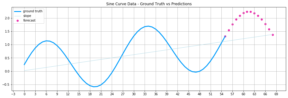
The line plot below illustrates the sample of a rising sine curve. The goal is to use the ground truth values (blue) to forecast several points in this curve (purple).
Traditional mathematical methods can resolve this function by decomposing it into constituent parts. Thus, we could easily foresee the further course of the curve. But in practice, the function might not be precisely periodic and change over a more extended period. Therefore, recurrent neural networks can achieve better results than traditional mathematical approaches, especially when they train on extensive data.
Also: Stock Market Prediction using Univariate Recurrent Neural Networks (RNN) with Python
Application Domains with Similar Time Series Forecasting Problems
A rising sine wave may sound like an abstract problem at first. However, similar issues are widespread. Imagine you are the owner of an online shop. The users who visit your shop and buy something fluctuate depending on the time and the weekday. For instance, there are fewer visitors at night, and on weekends, the number of visitors rises sharply. At the same time, the overall number of users increases over a more extended period as the shop becomes known to a broader audience. To plan the number of goods to be held in stock, you need to see the number of orders at any point in time over several weeks. It is a typical multi-step time series problem, and similar problems exist in various domains:
- Healthcare: e.g., forecasting of health signals such as heart, blood, or breathing signals
- Network Security: e.g., analysis of network traffic in intrusion detection systems
- Sales and Marketing: e.g., forecasting of market demand
- Production demand forecasting: e.g., for power consumption and capacity planning
- Prediction and filtering of sensor signals, e.g., of audio signals
A time series forecasting problem: predicting sine curve data
Recurrent Neural Networks for Time Series Forecasting
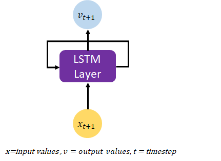
The model used in this article is a recurrent neural network with Long short-term memory (LSTM) layers. Unlike feedforward neural networks, recurrent networks with LSTM layers have loops to pass output values from one training instance to the next. LSTM layers are a powerful and widely-used tool for deep learning, and they work particularly well for time series data. By using LSTM layers, it is possible to train machine learning models that can make accurate predictions based on time series data, which can be useful for a wide range of applications, including finance, weather forecasting, and many others.
The Training Process of a Recurrent Neural Network
When training neural networks, the process typically involves multiple epochs, where an epoch refers to a single pass through the entire training dataset. During each epoch, the neural network receives the entire training data and adjusts its weights accordingly through forward and backward propagation. The batch size, which determines the number of examples passed through the network at once, also affects how the weights are updated between neurons.
It’s important to note that one epoch is usually not enough for the model to learn the underlying patterns and relationships in the data, leading to underfitting and poor performance in prediction tasks. Hence, multiple epochs are often needed to fine-tune the network and improve its predictive capabilities. However, care must be taken not to overfit the model by choosing too many epochs. Overfitting occurs when the model becomes too complex and performs well on the training data but poorly on any other data, resulting in poor generalization.
To avoid overfitting, we can employ various techniques such as early stopping, where the training process is stopped when the validation loss begins to increase, indicating that the model is overfitting. Another method is to use regularization techniques such as L1 or L2 regularization, dropout, or data augmentation to prevent overfitting and improve the model’s generalization capabilities.

Functioning of an LSTM layer
An LSTM (Long Short-Term Memory) layer is a specialized type of recurrent neural network (RNN) layer that is specifically designed for processing and making predictions based on time series data. Unlike traditional RNNs, which suffer from the vanishing gradient problem, LSTM layers can maintain a memory of past events and selectively use this memory to make predictions about future events.
LSTM layers accomplish this by incorporating several unique mechanisms, such as gates and cell states. The gates control the flow of information into and out of the cell, while the cell state represents the memory of the network. These mechanisms work together to enable LSTM layers to learn and make predictions based on long-term dependencies in the data, which is a characteristic of many time series datasets.
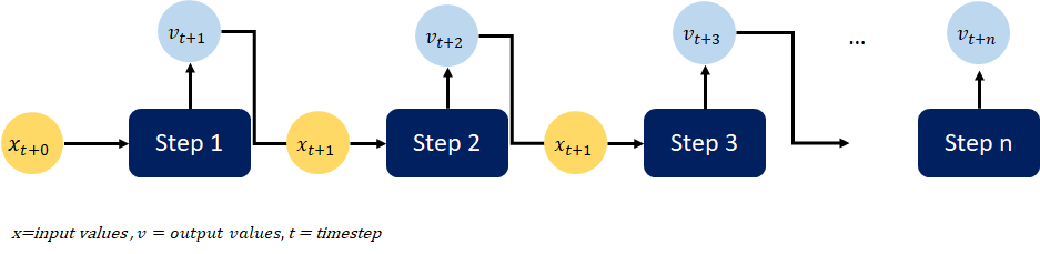
One of the key advantages of using LSTM layers for time series forecasting is their ability to generate predictions for multiple timesteps. This is achieved by iteratively reusing the model outputs from the previous training run as input for the next prediction step. This approach, known as a rolling forecast, allows the model to make accurate predictions for multiple time steps into the future.
Functioning of an LSTM layer
LSTM Components
To understand how an LSTM layer works, it is helpful to think about the layer as consisting of several different components, each of which has a specific role in the overall operation of the layer. These components include the following:
- Input gate: The input gate controls which information from the input data will be passed on to the cell state. The input gate uses a sigmoid activation function to determine which information should be retained and which should be discarded.
- Forget gate: The forget gate controls which information from the cell state will be discarded. The forget gate uses a sigmoid activation function to determine which information should be forgotten and which should be retained.
- Cell state: The cell state is a vector that contains the information that is retained by the LSTM layer. This information is updated at each time step based on the input from the input gate and the forget gate.
- Output gate: The output gate controls which information from the cell state will be passed on to the output of the LSTM layer. The output gate uses a sigmoid activation function to determine which information should be retained and which should be discarded.
This article uses LSTM layers combined with a rolling forecast approach to predict the course of a sinus curve with a linear slope. The result is a multi-step time series forecast.
Creating a Rolling Multi-Step Time Series Forecast in Python
In this tutorial, we will explore the process of creating a rolling multi-step forecast using Python. Our dataset for this exercise will be a synthetically generated rising sine curve, which we will use to demonstrate the principles of multi-step time series forecasting.
By following the steps outlined in this tutorial, you will gain a comprehensive understanding of the process involved in multi-step time series forecasting. This will include techniques for data preprocessing, feature engineering, and model selection.
To get started, we have made the code available on our GitHub repository. You can easily access and follow along with the tutorial by downloading the code and running it on your local machine. This will enable you to experiment with different parameters and modify the code to suit your specific requirements.
Prerequisites
Before starting the coding part, make sure that you have set up your Python 3 environment and required packages. If you don’t have an environment yet, you can follow this tutorial to set up the Anaconda environment.
Also, make sure you install all required packages. In this tutorial, we will be working with the following standard packages:
In addition, we will be using Keras(2.0 or higher) with Tensorflow backend and the machine learning library Scikit-learn.
You can install packages using console commands:
- pip install
- conda install
(if you are using the anaconda packet manager)
Step #1 Generating Synthetic Data
We begin by loading the required packages and creating a synthetic dataset. The synthetic data contains 300 values of the sinus function combined with a slight linear upward slope of 0.02. The code below creates the data and visualizes it in a line plot.
# A tutorial for this file is available at www.relataly.com

import math
import numpy as np
import pandas as pd
import matplotlib.pyplot as plt
from tensorflow.keras.models import Sequential
from tensorflow.keras.layers import LSTM, Dense, TimeDistributed, Dropout, Activation
from sklearn.preprocessing import RobustScaler
from sklearn.metrics import mean_absolute_error
import tensorflow as tf
import seaborn as sns
sns.set_style('white', { 'axes.spines.right': False, 'axes.spines.top': False})

# check the tensorflow version and the number of available GPUs
print('Tensorflow Version: ' + tf.__version__)
physical_devices = tf.config.list_physical_devices('GPU')
print("Num GPUs:", len(physical_devices))

# Creating the synthetic sinus curve dataset
steps = 300
gradient = 0.02
list_a = []
for i in range(0, steps, 1):
    y = round(gradient * i + math.sin(math.pi * 0.125 * i), 5)
    list_a.append(y)
df = pd.DataFrame({"sine_curve": list_a}, columns=["sine_curve"])

# Visualizing the data
fig, ax1 = plt.subplots(figsize=(16, 4))
ax1.xaxis.set_major_locator(plt.MaxNLocator(30))
plt.title("Sinus Data")
sns.lineplot(data=df[["sine_curve"]], color="#039dfc")
plt.legend()
plt.show()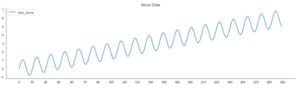
The signal curve oscillates and is steadily moving upward.
Step #2 Preprocessing
Next, we preprocess the data to bring it into the shape required by our neural network model. Running the code below will perform the following tasks:
- Scale the data to a standard range.
- Partition the data into multiple periods with a predefined sequence length. Each partition series contains 110 data points. The number of steps needs to match the number of neurons in the first layer of the neural network architecture.
- Split the data into two separate datasets for training and testing.
data = df.copy()

# Get the number of rows in the data
nrows = df.shape[0]

# Convert the data to numpy values
np_data_unscaled = np.array(df)
np_data_unscaled = np.reshape(np_data_unscaled, (nrows, -1))
print(np_data_unscaled.shape)

# Transform the data by scaling each feature to a range between 0 and 1
scaler = RobustScaler()
np_data_scaled = scaler.fit_transform(np_data_unscaled)

# Set the sequence length - this is the timeframe used to make a single prediction
sequence_length = 110

# Prediction Index
index_Close = 0

# Split the training data into train and train data sets
# As a first step, we get the number of rows to train the model on 80% of the data
train_data_len = math.ceil(np_data_scaled.shape[0] * 0.8)

# Create the training and test data
train_data = np_data_scaled[0:train_data_len, :]
test_data = np_data_scaled[train_data_len - sequence_length:, :]

# The RNN needs data with the format of [samples, time steps, features]
# Here, we create N samples, sequence_length time steps per sample, and 6 features
def partition_dataset(sequence_length, data):
    x, y = [], []
    data_len = data.shape[0]
    for i in range(sequence_length, data_len):
        x.append(data[i-sequence_length:i,:]) #contains sequence_length values 0-sequence_length * columsn
        y.append(data[i, index_Close]) #contains the prediction values for validation (3rd column = Close),  for single-step prediction

    # Convert the x and y to numpy arrays
    x = np.array(x)
    y = np.array(y)
    return x, y

# Generate training data and test data
x_train, y_train = partition_dataset(sequence_length, train_data)
x_test, y_test = partition_dataset(sequence_length, test_data)

# Print the shapes: the result is: (rows, training_sequence, features) (prediction value, )
print(x_train.shape, y_train.shape)
print(x_test.shape, y_test.shape)

# Validate that the prediction value and the input match up
# The last close price of the second input sample should equal the first prediction value
print(x_test[1][sequence_length-1][index_Close])
print(y_test[0])
(130, 110, 1) (130,)
(60, 110, 1) (60,)
0.599655121905751
0.599655121905751Step #3 Preparing Data for the Multi-Step Time Series Forecasting Model
Now that we have prepared the synthetic data, we need to determine the architecture of our neural network. There are no clear guidelines available on how to configure a neural network. Most problems are unique, and the model settings depend on the nature and extent of the data. Thus, configuring LSTM layers can be a real challenge.
3.1 Overview of Model Parameters
Finding the optimal configuration is often a process of trial and error. Below you find a list of model parameters with which you can experiment:
Keras model parameters used in this tutorial epoch: An epoch is an iteration over the entire x_train and y_train data provided. Batch_size: Number of samples per gradient update. If unspecified, batch_size is 32. Activation: Mathematical equations determine whether a neuron in the network should activate (“fired”) or not. Input_shape: Tensor with shape: (batch_size, …, input_dim). Input_len: the length of the generated input sequence. Return_sequences: If set to false, the layer will return the final output in the output sequence. If true, the layer returns the entire series. Loss: The loss function tells the model how to evaluate its performance so that the weights can be updated to reduce the loss on the following evaluation. Optimizer: Every time a neural network finishes processing a batch through the network and generates prediction results, the optimizer decides how to adjust weights between the nodes.
Source: keras.io/layers/recurrent - view the Keras documentation for a complete list of parameters.
3.2 Choosing Model Parameters
Finding a suitable architecture for a neural network is not easy and requires a systematic approach. A common practice is to start with an established standard architecture. We can then change the model parameters slightly and record the configurations and outcomes. We can also automate configuring and testing the model (Hyperparameter Tuning). Still, because this is not the focus of this article, we will use a manual approach.
We start with five epochs, a batch_size of 1, and configure our recurrent model with one LSTM layer with 110 neurons, corresponding to a data slice of 110 input values. In addition, we add a dense layer that provides us with a single output value.
# Configure the neural network model
epochs = 12; batch_size = 1;

# Model with n_neurons = inputshape Timestamps, each with x_train.shape[2] variables
n_neurons = x_train.shape[1] * x_train.shape[2]
model = Sequential()
model.add(LSTM(n_neurons, return_sequences=True, input_shape=(x_train.shape[1], 1)))
model.add(LSTM(n_neurons, return_sequences=False))
model.add(Dense(5))
model.add(Dense(1))
model.compile(optimizer="adam", loss="mean_squared_error")
Step #3 Training the Prediction Model
Now that we have defined the architecture of our recurrent neural network, the next step is to train the model. Training the model involves using a training dataset to adjust the weights and biases of the network so that it can make accurate predictions on new data. This process is done using an optimization algorithm, such as gradient descent, to minimize the difference between the predicted values and the true values.
Training can be time-consuming, especially for large datasets or complex models, and the amount of time it takes may vary depending on the performance of your computer. The complexity of our model is relatively low, and we only use five training epochs. It should thus only take a couple of minutes to train the model.
It is important to monitor the training process to ensure that the model is learning effectively and to identify any potential issues or problems. Once the training is complete, we can test the model on a separate test dataset to evaluate its performance.
# Train the model
history = model.fit(x_train, y_train, batch_size=batch_size, epochs=epochs)
Epoch 1/12
130/130 [==============================] - 7s 28ms/step - loss: 0.0544
Epoch 2/12
130/130 [==============================] - 4s 27ms/step - loss: 0.0041
Epoch 3/12
130/130 [==============================] - 4s 28ms/step - loss: 3.5105e-04
Epoch 4/12
130/130 [==============================] - 4s 28ms/step - loss: 4.3903e-05
Epoch 5/12
130/130 [==============================] - 4s 28ms/step - loss: 5.9422e-05
Epoch 6/12
130/130 [==============================] - 4s 28ms/step - loss: 5.7988e-05
Epoch 7/12
130/130 [==============================] - 4s 28ms/step - loss: 8.3814e-04
Epoch 8/12
130/130 [==============================] - 4s 28ms/step - loss: 1.9122e-04
Epoch 9/12
130/130 [==============================] - 4s 28ms/step - loss: 0.0014
Epoch 10/12
130/130 [==============================] - 4s 29ms/step - loss: 0.0114
Epoch 11/12
130/130 [==============================] - 4s 28ms/step - loss: 0.0013
Epoch 12/12
130/130 [==============================] - 4s 28ms/step - loss: 3.4571e-05Step #4 Predicting a Single-step Ahead
We continue by making single-step predictions based on the training data. Then we calculate the mean squared error and the median error to measure the performance of our model.
# Reshape the data, so that we get an array with multiple test datasets
x_test_np = np.array(x_test)
x_test_reshape = np.reshape(x_test_np, (x_test_np.shape[0], x_test_np.shape[1], 1))

# Get the predicted values
y_pred = model.predict(x_test_reshape)
y_pred_unscaled = scaler.inverse_transform(y_pred)
y_test_unscaled = scaler.inverse_transform(y_test.reshape(-1, 1))

# Mean Absolute Error (MAE)
MAE = mean_absolute_error(y_test_unscaled, y_pred_unscaled)
print(f'Median Absolute Error (MAE): {np.round(MAE, 2)}')

# Mean Absolute Percentage Error (MAPE)
MAPE = np.mean((np.abs(np.subtract(y_test_unscaled, y_pred_unscaled)/ y_test_unscaled))) * 100
print(f'Mean Absolute Percentage Error (MAPE): {np.round(MAPE, 2)} %')

# Median Absolute Percentage Error (MDAPE)
MDAPE = np.median((np.abs(np.subtract(y_test_unscaled, y_pred_unscaled)/ y_test_unscaled)) ) * 100
print(f'Median Absolute Percentage Error (MDAPE): {np.round(MDAPE, 2)} %')
Out: me: 0.0223, rmse: 0.0206Both the mean error and the squared mean error are pretty small. As a result, the values predicted by our model are close to the actual values of the ground truth. Even though it is unlikely because of the small number of epochs, it could still be that the model is over-fitting.
Step #5 Visualizing Predictions and Loss
Next, we look at the quality of the training predictions by plotting the training predictions and the actual values (i.e., ground truth).
# Visualize the data
#train = df[:train_data_len]
df_valid_pred = df[train_data_len:]
df_valid_pred.insert(1, "y_pred", y_pred_unscaled, True)

# Create the lineplot
fig, ax1 = plt.subplots(figsize=(32, 5), sharex=True)
ax1.tick_params(axis="x", rotation=0, labelsize=10, length=0)
plt.title("Predictions vs Ground Truth")
sns.lineplot(data=df_valid_pred)
plt.show()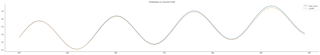
The smaller the area between the two lines, the better our model predictions. So we can tell from the plot that the predictions are not entirely wrong. We also check the learning path of the regression model.
# Plot training & validation loss values
fig, ax = plt.subplots(figsize=(10, 5), sharex=True)
sns.lineplot(data=history.history["loss"])
plt.title("Model loss")
plt.ylabel("Loss")
plt.xlabel("Epoch")
ax.xaxis.set_major_locator(plt.MaxNLocator(epochs))
plt.legend(["Train"], loc="upper left")
plt.grid()
plt.show()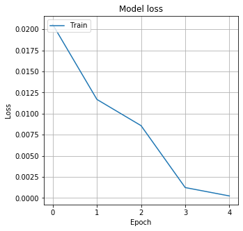
The loss drops quickly, and after five epochs, the model seems to have converged.
Step #6 Rolling Forecasting: Creating a Multi-step Time Series Forecast
Next, we will generate the rolling multi-step forecast. This approach is different from a single-step approach in that we predict several points of a signal within a prediction window and not just a single value. However, the prediction quality decreases over more extended periods because reusing predictions creates a feedback loop that amplifies potential errors over time.
Also: Measuring Regression Errors with Python
The forecasting process begins with an initial prediction for a single time step. After that, we add the predicted value to the input values for another projection, and so on. In this way, we create the rolling forecast with multiple time steps.
# Settings and Model Labels
rolling_forecast_range = 30
titletext = "Forecast Chart Model A"
ms = [
    ["epochs", epochs],
    ["batch_size", batch_size],
    ["lstm_neuron_number", n_neurons],
    ["rolling_forecast_range", rolling_forecast_range],
    ["layers", "LSTM, DENSE(1)"],
]
settings_text = ""
lms = len(ms)
for i in range(0, lms):
    settings_text += ms[i][0] + ": " + str(ms[i][1])

    if i < lms - 1:
        settings_text = settings_text + ",  "

# Making a Multi-Step Prediction
# Create the initial input data
new_df = df.filter(["sine_curve"])
for i in range(0, rolling_forecast_range):
    # Select the last sequence from the dataframe as input for the prediction model
    last_values = new_df[-n_neurons:].values

    # Scale the input data and bring it into shape
    last_values_scaled = scaler.transform(last_values)
    X_input = np.array(last_values_scaled).reshape([1, 110, 1])
    X_test = np.reshape(X_input, (X_input.shape[0], X_input.shape[1], 1))

    # Predict and unscale the predictions
    pred_value = model.predict(X_input)
    pred_value_unscaled = scaler.inverse_transform(pred_value)

    # Add the prediction to the next input dataframe
    new_df = pd.concat([new_df, pd.DataFrame({"sine_curve": pred_value_unscaled[0, 0]}, index=new_df.iloc[[-1]].index.values + 1)])
    new_df_length = new_df.size
forecast = new_df[new_df_length - rolling_forecast_range : new_df_length].rename(
    columns={"sine_curve": "Forecast"}
)
We can plot the forecast together with the ground truth.
#Visualize the results
validxs = df_valid_pred.copy()
dflen = new_df.size - 1
dfs = pd.concat([validxs, forecast], sort=False)
dfs.at[dflen, "y_pred_train"] = dfs.at[dflen, "y_pred"]
dfs

# Zoom in to a closer timeframe
df_zoom = dfs[dfs.index > 200]

# Visualize the data
fig, ax = plt.subplots(figsize=(16, 5), sharex=True)
ax.tick_params(axis="x", rotation=0, labelsize=10, length=0)
ax.xaxis.set_major_locator(plt.MaxNLocator(rolling_forecast_range))
plt.title('Forecast And Predictions (y_pred)')
sns.lineplot(data=df_zoom[["sine_curve", "y_pred"]], ax=ax)
sns.scatterplot(data=df_zoom[["Forecast"]], x=df_zoom.index, y='Forecast', linewidth=1.0, ax=ax)
plt.legend(["x_train", "y_pred", "y_test_rolling"], loc="lower right")
ax.annotate('ModelSettings: ' + settings_text, xy=(0.06, .015),  xycoords='figure fraction', horizontalalignment='left', verticalalignment='bottom', fontsize=10)
plt.show()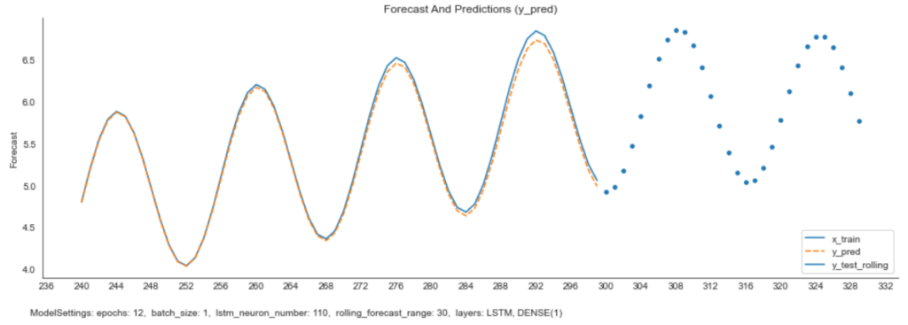
The model learned to predict the periodic movement of the curve and thus succeeds in modeling its further course. However, the amplitude of the predicted curve increases over time, which increases the prediction errors.
Step #7 Comparing Results for Different Parameters
There is plenty of room to improve the forecasting model further. So far, our model seems not to consider that the amplitude of the sinus curve is gradually increasing. Over time, errors are amplified, leading to a growing deviation from the ground truth signal.
We can improve the model by changing the model parameters and the model architecture. However, I would not recommend changing them one at a time.
I tested several model configurations with varying epochs and neuron numbers/sample sizes to further optimize the model. Parameters such as Batch_size (=1), the timeframe for the forecast (=30 timesteps), and the model architecture (=1 LSTM Layer, 1 DENSE Layer) were left unchanged. The illustrations below show the results:
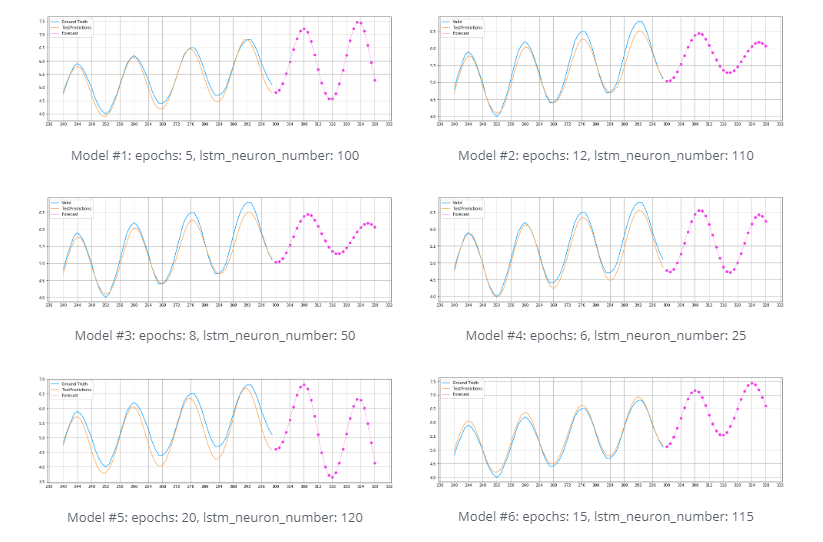
Different designs of the rolling time series forecasting model
The model that looks most promising is model #6. This model considers both the periodic movements of the sinus curve and the steadily increasing slope. The configuration of this model uses 15 epochs and 115 neurons/sample values.
Errors are amplified over more extended periods when they enter a feedback loop. For this reason, we can see in the graph below that the prediction accuracy decreases over time.
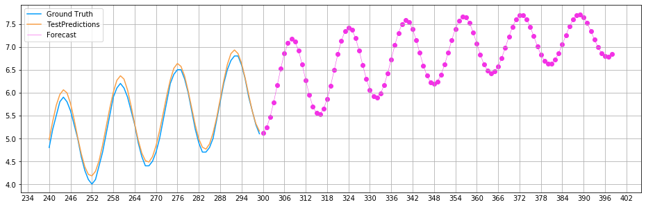
Long-time multi-step forecast (model #6)
Summary
In this tutorial, we have created a rolling time-series forecast for a rising sine curve. A multi-step forecast helps better understand how a signal will develop over a more extended period. Finally, we have tested and compared different model variants and selected the best-performing model.
There are several ways to improve model accuracy further. For example, the current network architecture was kept simple and only had a single LSTM layer. Consequently, we could try to add additional layers. Another possibility is to experiment with different hyperparameters. For example, we could increase the training epochs and use dropout to prevent overfitting. In addition, we could experiment with other activation functions. Feel free to try it out.
I hope this article was helpful. If you have questions remaining, let me know in the comments.
Another forecasting approach is to train a neural network model that predicts multiple outputs per input batch. Another relataly article demonstrates how this multi-output regression approach works: Stock Market Prediction - Multi-output regression in Python.
Also, consider non-neural network approaches to time series forecasting, such as ARIMA, which can achieve great results too.
Sources and Further Reading
The links above to Amazon are affiliate links. By buying through these links, you support the Relataly.com blog and help to cover the hosting costs. Using the links does not affect the price.


2 Commentsarchived from the original site